Performance Evaluation of Context-Dependent Lexical Information

Normalization Using Word Embedding Techniques

Amit Shukla and Rajendra Gupta

Rabindranath Tagore University, Bhopal, India

Keywords: Word Embeddings, Context-Dependent Lexical Information, Normalization.

Abstract: The word embedding is a type of word representation that allows machine learning algorithms to recognise

words that have the same meaning. The majority of lexical normalization approaches work at the character

level. While character-level models use far less memory than word-level models, they have a proclivity for

predicting slightly erroneous character sequences, resulting in lower accuracy. Since, the misspelt words do

not have corresponding word embedding vectors unless the embedding model is trained on the training corpus

itself, which is often much smaller than the corpora used for embedding training, word-level models are rarely

employed for lexical normalization. The usefulness of these cutting-edge embedding models for lexical

normalization of small text data has yet to be determined. Furthermore, practically the lexical normalization

research is focused on social media applications. The paper presents the performance evaluation of context

dependent lexical information normalization using word embedding technique and found that the word-level

model is better in predicting a word that needs to be normalized. The result shows the accuracy percentage is

around 75 which is about 2 percent better than the earlier proposed normalization methods.

1 INTRODUCTION TO WORD

EMBEDDINGS

The word embeddings is a feature learning technique

that uses probabilistic models, dimension reduction,

or neural networks on the word co-occurrence vector

matrix to map words into real-number vectors.

Consider the phrase 'Tiger,' which is context

independent, but is context dependent when we say

'The Tiger is dangerous' or 'The Tiger may be

harmful.'

Because of the word embeddings overcome the

drawbacks of Bag of Words and other additional

procedures to be implement, it is more effective and

unique than other strategies (Kong et.al., 2021). A

few of the reasons why word embedding is superior

to other techniques are as follows:

▪ Word Embedding outperforms other NLP

algorithms because it decreases the dataset's

dimensions more effectively.

▪ It is faster at training than other methods since

it doesn't require as much weight as other

methods do, or it takes less time to execute.

▪ Linguistic analysis, another name for NLP, is a

technique that has a greater grasp of words and

sentences than other NLP methods.

▪ It is preferable for computational reasons

because it does not adopt the Sparse matrix's

methodology.

The word embeddings can be applied on the

following:

▪ Finding Similar Words:

▪ Text Classification:

▪ Document Clustering:

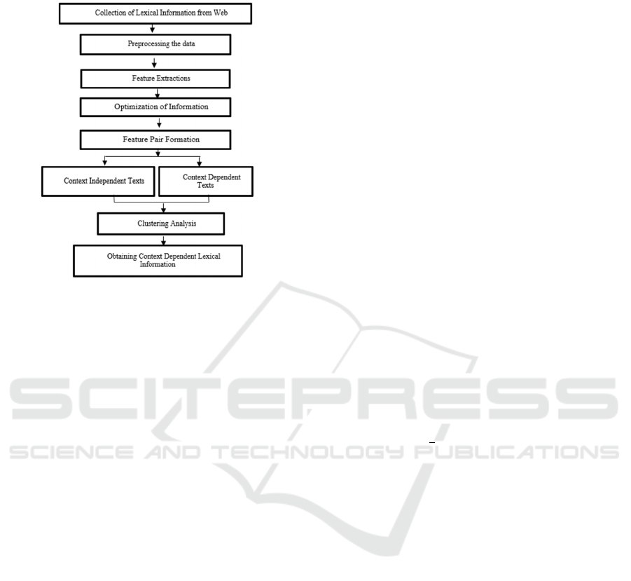
The process of restoring well-formed tokens in a

dataset to their canonical form is known as lexical

normalization (word normalization). It's a crucial step

in practically every natural language processing

activity, including entity recognition, sentiment

analysis, text classification, and automatic question

answering (Chow et.al., 2020).

Context-dependent embeddings have recently

become more popular due to this property. The

learning strategies for context-dependent word

embedding have essentially developed into two

groups as research has done (Kamakshi et.al., 2020).

Keeping the embedding layer as the single variant

but with the others as invariants is an essential

component of comparison experiments for

Shukla, A. and Gupta, R.

Performance Evaluation of Context-Dependent Lexical Information Normalization Using Word Embedding Techniques.

DOI: 10.5220/0012604000003739

Paper published under CC license (CC BY-NC-ND 4.0)

In Proceedings of the 1st International Conference on Artiﬁcial Intelligence for Internet of Things: Accelerating Innovation in Industry and Consumer Electronics (AI4IoT 2023), pages 615-619

ISBN: 978-989-758-661-3

615

successfully testing their impact. This inspires the

objectives of our work.

Figure 1: An Illustration of Word level Lexical

Normalization Model.

2 MODEL ARCHITECTURE

Using a bidirectional gated recurrent unit, we present

a word-level Lexical Normalization Model (LNM).

The LNM is a more straightforward version of the

Neural Text Normalization Model (NTNM). When

predicting the right form of the word, the Bi-LNM, as

opposed to a unidirectional LNM, considers both

forward and backward contexts. This is important

because the words that precede it ("he turned l") and

follow it ("l leg was damaged") can determine the

correct form of a word, such as "l" (whose correct

form may be "left"). It's often determined by the

words that come before and after it ("he damaged his

l leg").

The model receives a sequence of tokens as input

and predicts a sequence of labels as output, as shown

in Fig.1. Each input token has a single output token

that corresponds to the right form of that token. A

special label is used to denote words that are already

in their right form, similar to how a special label is

used to denote words that are already in their correct

form. This speeds up training by lowering the number

of viable labels to predict, while also boosting

performance by lowering the number of infrequently

occurring labels. The figure shows how the original

shorthand token "l" is normalized to "left," whereas

the rest of the tokens in the sentence don't need to be

normalized and are thus labeled (Akokaet.al., 2020).

The model can also be applied to individual

characters. It can anticipate the correct character

instead of guessing the correct form of each word in

a phrase.

3 WORD EMBEDDING

SEMANTIC

Knowing a word's semantics and context is necessary

for representing it because a word's meaning changes

depending on the context in which it is used. For

illustration, let's look at the term "bank." There are

numerous meanings of term ‘bank’. A definition of a

word is a financial institution, while another defines

it as land next to water. If the term "bank" appears in

a phrase along with words like "money,"

"government," "treasury," "interest rates,"

etc.(Mouza et.al. 2019).

The Word2Vec is a popular word embedding

model that combines two training models: Skip-gram

and Continuous Bag Of Words (CBOW). Skip-gram

seeks to predict the surrounding context of a word,

whereas CBOW predicts a word given a surrounding

context. The skip-gram model seeks to maximize the

log likelihood of all words predicted in a context

window of size w surrounding word -

𝑤

𝑇











𝑙𝑜𝑔 𝑝



𝑤





The FastText works in the same way as

Word2Vec's skip-gram variation, but instead

represents each word as a bag of character n-grams

alongside the word. A modified scoring function is

used to evaluate the model's predictions:

𝑠



𝑤,𝑐





∈

𝑍





𝑣



where w denotes a word, G

is the set of n-grams

that appear in w, G denotes the size of each n-gram,

and Z

denotes the vector representation of each n-

gram g.

The ELMo creates embeddings from learned

bidirectional language model functions (Bi-LM).

Two recurrent LSTMs are used in a Bi-LM. Based on

the chance of each token appearing t given a sequence

of preceding tokens, the forward model computes the

probability of a context window of tokens (t

; t

;

……. ;t

AI4IoT 2023 - First International Conference on Artiﬁcial Intelligence for Internet of things (AI4IOT): Accelerating Innovation in Industry

and Consumer Electronics

616

𝑝



𝑡



,𝑡



,………….𝑡





 





𝑝



𝑡



,𝑡



,………….𝑡





The backward model works in the same way as

the forward model, but predicts the previous token

from a sequence of future tokens. These two models

are combined in ELMo, which maximizes the log

likelihood in both directions.

The F-Measure, which is derived from

information retrieval, assesses the accuracy of

pairwise relationship judgments and is also known as

pairwise F-Measure. The F- Measure is calculated as :

𝐹





𝛽



1𝑃𝑅

𝛽



𝑃𝑅

Where β is a variable function.

Propositions, pronouns, and articles are

commonly used stop words that do not contribute in

clustering. Hence, they are eliminated from dataset

texts. Following that, the pre-processed dataset is read

as vectors containing numerical values for Term

Frequency-Inverse Document Frequency (TF-IDF)

for each word (Term) in the dataset. Term Frequency

(TF) is the number of times a word (Term) appears in

a document, and inverse Document Frequency (DF)

is the log of the ratio of the total number of documents

in the dataset to the number of documents containing

that word. The TF-IDF matrix is the product of these

two measurements, TF and IDF as shown below:

After that TF-IDF matrix is converted into single

frequency.

TF-IDF informs the importance of a document's

terms. A word may appear in a document more

frequently if it is longer than it is shorter(Parket.al.,

2019).

4 EXPERIMENTAL ANALYSIS

A short text lexical normalization dataset for lexical

normalisation is available on UCI Repository ML

database. It's an annotated version of the Twitter

dataset, which is a combination of structured and

unstructured data on number of tweets (Gómez-

Hidalgo et.al. 2014). We construct embeddings using

four-word embedding models to test our word-level

model: Word2Vec, FastText, ELMo, and BERT. The

Bi-LNM word-level model takes the embedding

vectors from all embedding models except BERT as

input. As proposed by the BERT publication, the

BERT embeddings are fed via a single feed-forward

layer followed by a softmax classifier. With an

embedding dimension of 512 and a window size of

10, the Word2Vec and FastText models were trained.

The ELMo was also trained with a 512-embedding-

dimensions.

Word-level Lexical Normalization Evaluation

Process

The three types of embedding techniques are

investigated and compared. For the dataset, we may

copy any unstructured data as a corpus and paste it as

a “.txt” file. Following are the normalization steps:

Step 1 Importing important libraries and

initializing the dataset.

Step 2

- Pre-processing of data,

- Substituting regular expressions

- Removing Stop-words

Step 3 Assigning unique data values to vocabulary

Step 4 Implementing the one-hot vector encoding

to preprocess categorical features in the machine

learning model.

Step 5 Assigning X and Y for training and testing,

and then splitting them.

Step 6 Implementing Word embedding

5 OBSERVATIONS ON

WORD-LEVEL LEXICAL

NORMALIZATION

TECHNIQUE (WLNT)

Table 1 Illustrates the results of the word-level model

after applying the co-occurrence strategies to

initialize the embeddings. We utilize Principle

Component Analysis (PCA) to minimize the length of

each embedding vector. There isn't much of a

difference in the results of each co-occurrence model.

In each iteration, the word-level model

outperforms both the character-level and the word-

level models. Despite not conducting character-level

normalisation like most state-of-the-art lexical

normalization systems, the word-level model's

capacity to use contextual information, paired with

the strong word representations from ELMo, allows it

to outperform other models. Overall, it's obvious that,

Performance Evaluation of Context-Dependent Lexical Information Normalization Using Word Embedding Techniques

617

with the correct embedding technique, word-level

lexical normalization has a lot of potential.

Table 1: F1 score of Word-level Lexical Normilation Model

(LNM) on each of the datasets when the embedding layer is

initialized with one of three co-occurrence embedding

techniques.

One-hot Cumulative TF-IDF F1-Score

No PCA

Twitter

Aus Acc

US Acc

0.6447

0.7348

0.7240

0.6475

0.7333

0.7503

0.6271

0.7236

0.7364

0.6475

0.7348

0.7503

After PCA

Twitter

Aus Acc

US Acc

0.6377

0.7187

0.7480

0.6356

0.7023

0.7567

0.6298

0.7326

0.7385

0.6377

0.7326

0.7567

6 PERFORMANCE ANALYSIS

WITH EXISTING SYSTEMS

The F1-Scores are consistently improved by

dictionary normalisation, which reflects the findings.

For the character-level model, the flagger module

works fine, but not for the word-level model (Trieu

et.al. 2018). This shows that the word-level model is

actually better than the flagger at predicting whether

a word needs to be normalised, which is surprising

given the flagger's sole purpose.

Table 2: A performance Comparison of the Word-level

WLNT against Existing Lexical Normalization Techniques.

Model F1-Score

Random Fores

0.7321

Lexicon 0.7172

Word-level WLNT 0.7552

Deep Contextual (NTNM) 0.7075

Deep Encodin

0.7049

For the Twitter dataset, Table 2 compares the F-Score

of the earlier proposed model (Wordlevel with ELMo

Embeddings) to the top four lexical normalization

approaches in the earlier study. For the normalization

of Twitter data, the method surpasses all known deep-

learning-based algorithms. With the exception of the

Lexicon model, the current systems shown in the

table did not have access to external unlabeled

Twitter data as part of the competition.

7 CONCLUSIONS

The idea of word embedding is a type of word

representation that allows machine learning

algorithms to recognise words that have the same

meaning. It is a feature learning technique that uses

probabilistic models, dimension reduction, or neural

networks on the word co-occurrence vector matrix to

map words into real-number vectors.The paper

presents the performance evaluation of context

dependent lexical information normalization using

word embedding technique and found that the word-

level model is better in predicting a word that needs

to be normalized. The result shows the accuracy

percentage 75.52 which is about better than as

compared to earlier proposed normalization methods

like Random Forest, Lexicon, Deep Contextual and

Deep encoding methods. The F1-scores are

consistently improved by the proposed normalization

process, which reflects the findings.

REFERENCES

Kong J., Li W., Liu Z., Liao B., Qiu J., Hsieh C.Y., Cai Y.,

Zhang S. (October 2021) Fast Extraction of Word

Embedding from Q-contexts, CIKM '21: Proceedings

of the 30th ACM Int. Conf. on Information &

Knowledge Management, 873–882

ChowR., GolleP. and StaddonJ. (2020)Detecting privacy

leaks using corpus-based association rules, in:

Proceeding of the 14th ACM SIGKDD Int. Conf. on

Knowledge Discovery and Data Mining–KDD-08, 234-

238.

KamakshiP., BabuA.V.(2020) Automatic detection of

lexical attribute in PPDM”, in: 2012 IEEE Inter. Conf.

on Computational Intelligence and Computing

Research, 1–5.

AkokaJ., Comyn-WattiauI., MouzaC.D., FadiliH.,

LammariN., MetaisE., CherfiS.S.-S. (2020) “A

Semantic Approach for Semi-Automatic Detection of

Lexical Data”, Information Resource Management, J.

27 (4), 23–44.

MouzaC.D., MétaisE., LammariN., AkokaJ., AubonnetT.,

Comyn-WattiauI., FadiliH. andCherfiS.S.-S.d. (2019).

Towards an automatic detection of lexical information

in a database. Second Inter. Conf. on Advances in

Databases, Knowledge and Data Applications.

HeniH. andGargouriF.(2019). Towards an automatic

detection of lexical information in mongo database,

Adv. Int. Sys. Computer Intelligent System Design

Application, 138–146.

ParkJ.-s., KimG.-w. and LeeD. (2019). Sensitive data

identification in structured data through genner model

based on text generation and NER, in: Proceedings of

the 2020 International Conference on Computing,

Networks and Internet of Things, in: CNIOT2020,

Association for Computing Machinery, New York, NY,

USA, pp. 36–40.

TrieuL.Q., TranT.-N., TranM.-K. and TranM.-T. (2018).

Document sensitivity classification for data leakage

AI4IoT 2023 - First International Conference on Artiﬁcial Intelligence for Internet of things (AI4IOT): Accelerating Innovation in Industry

and Consumer Electronics

618

prevention with twitter-based document embedding and

query expansion, in: 13th International Conference on

Computational Intelligence and Security (CIS), pp.

537–542.

Gómez-HidalgoJ.M., Martín-AbreuJ.M., NievesJ.,

SantosI., BrezoF. andBringasP.G. (2014). Data leak

prevention through named entity recognition”, in: 2010

IEEE Second International Conference on Social

Computing, pp. 1129–1134.

Performance Evaluation of Context-Dependent Lexical Information Normalization Using Word Embedding Techniques

619