
Availability and Behavioral Analysis of Refrigerating Unit in Milk
Plant with Scheduling: A Case Study of Milk Plant Rohtak
Savita Grewal
*
and Pooja Bhatia
†
Department of Mathematics, Baba Mastnath University Asthal Bohar, Rohtak, Haryana, India
Keywords: MTSF, RPGT, Availability
Abstract: In the current investigation one have picked the Refrigeration Plant arranged in Rohtak District. A
refrigeration unit involves of four main mechanisms namely Compressor, Condenser, Expansion Device and
Evaporator. Refrigeration plants are thought to be only viable when all four units are in good operating
condition. When each of the four units is in good operating condition, the system operates at maximum
efficiency. When three out of four units are in good operating condition, it operates at a decreased capacity.
When two or more units flop, the system is in a failed condition. There are separate continuous failure and
repair rates for all four units. A single repairman is available 24*7. The results of the sensitivity analysis can
be used to validate or challenge existing models and assumptions about the system. The deep learning can
provide valuable insights into the factors that affect system performance, Accuracy (MTSF), Expected
Number of Inspections by the repair man, Busy Period and Availability of the System and results in show in
figures and using the table.
1 INTRODUCTION
This study uses RPGT to analyses the behavior of a
refrigeration unit in a milk processing plant in the
Rohtak region with two units A and B, a permanent
repairman who attends to the online units according
to the schedule, and a specialist repairman who is
called when one of the subsystems A has fewer units
than a threshold number 't' of units. There are two
different kinds of subsystems, A and B. In subsystem
"A," there are "m" online units with a pool of "n"
(fewer than m) units in cold standby, but subsystem
"B" has units in series, thus it fails when any of its
subunits fails, leading to the failure of the entire
system. In sub system ‘A’ online units remain
scheduled aimed at service/ repair single by single
and replaced through one of the standby units after
the pool. If number of good online units stand in the
variety, {m < i < t}, and number of online units in A
are left to less than a threshold number ‘t’, then the
subsystem A fails, hence the whole system is failed,
then a special repairman is entitled for repairing/
serving the failed units. Both types of equipment are
repaired or serviced by a permanent repairman, but
*
Research Scholar
†
Professor
subsystem B is given precedence in repairs. RPGT is
used to obtain expressions for System parameter
values. To compare the impact of various repair and
failure rates on the parameter values, graphs and
tables are created for each value. For the repair of
malfunctioning devices and in diminished stages,
there is just one repairman. The rates of failure are
exponentially distributed, while the rates of repair are
universal, independent, and distinct for various
operational units varying units have varying
capabilities. The fixes are flawless. As discussed, in
this paper Rohtak region have rich in milk production
as there are quite several milch animals, which is
further processed to produce several useful milk
products, one of such most useful product in our daily
life is milk which is used for drinking by humans of
all ages from infants to old persons. This milk is of
many types of generally full cream, toned and double
toned and is distributed and sold in the market of all
available different types of urban, semiurban, and
rural area located in the Rohtak region. In a
Refrigerating unit of Rohtak there two sets of pools,
one set of which is online i.e., which refrigerates the
milk
and other set is in cold standby made have a
170
Grewal, S. and Bhatia, P.
Availability and Behavioral Analysis of Refrigerating Unit in Milk Plant with Scheduling: A Case Study of Milk Plant Rohtak.
DOI: 10.5220/0012608800003739
Paper published under CC license (CC BY-NC-ND 4.0)
In Proceedings of the 1st International Conference on Artificial Intelligence for Internet of Things: Accelerating Innovation in Industry and Consumer Electronics (AI4IoT 2023), pages 170-177
ISBN: 978-989-758-661-3
Proceedings Copyright © 2024 by SCITEPRESS – Science and Technology Publications, Lda.
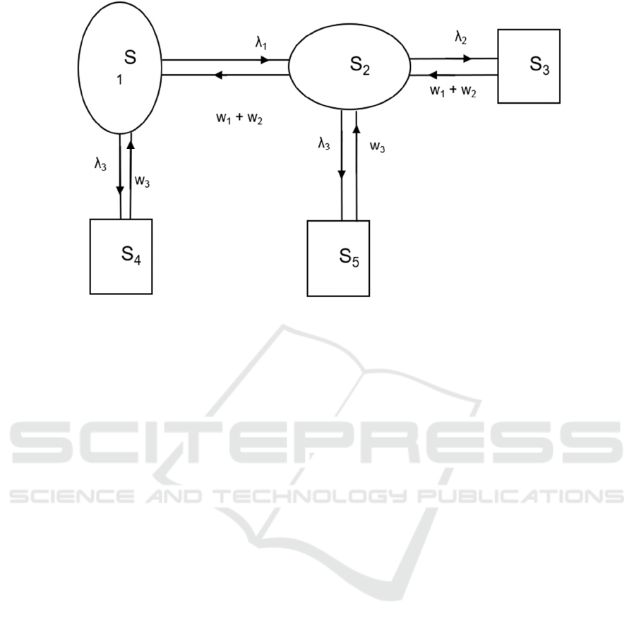
Figure 1: Transition Diagram.
certain number of units in the offline mode, online
spools are scheduled for a service and are made
offline after a fixed period and a spool from the
standby pool is mode online. (Shakuntla et al 2011)
discussed the behavior analysis of polytube using
supplementary variable procedure; the behavior of a
bread plant was examined by (Kumar et al. 2018). To
do a sensitivity analysis on a cold standby framework
made up of two identical units with server failure and
prioritized for preventative maintenance (Kumar et al.
2019) used RPGT, two halves make up the paper, one
of which is in use and the other of which is in cold
standby mode. The comparative analysis of the
subsystem failed simultaneously was discussed by
(Shakuntla et al. 2011). In a paper mill washing unit
(Kumar et al. 2019) investigated mathematical
formulation and behavior study. PSO was used by
(Kumari et al. 2021) to research limited situations.
Using a heuristic approach, (Rajbala et al. 2022)
investigated the redundancy allocation problem in the
cylinder manufacturing plant. The tables and graphs
are created using analytical cases, and they are then
discussed. Following the use of specific examples, the
effect is expressed using tables and graphs as well as
concluding remarks.
1.1 Working of the System
There are two subsystems A and B in milk plant of
Refrigerating Unit. In unit ‘A’ their ‘m’ online and
‘n’ units in cold standby mode switched in with online
unit’s pool to online units by a perfect switch over
device as per a schedule one by one. There is one
permanent that is continually available. To repair the
unsuccessful unit (s) of sub system A, the failure rate
of subsystem ‘A’ is λ
1
, if number of subunits in it are
online and if the number of online units in subsystem
‘A’ are less than the threshold ‘t’, then the
arrangement worked in reduced capacity shown in
transition diagram as S
2
, further if the number of
online units in ‘A’ are less than a threshold ‘t’ then it
fails at a failure rate λ
2
. The unit ‘B’ has subunits in
series, so if one of the subunits in ‘B’ flops, then the
unit ‘B’ fails whose failure rate is λ
3
. A specials
repairman is called in if in subsystem ‘A’ there are
less than ‘t’ online units to keep the system available,
so the combined repair rate of two repairman will be
w
1
+w
2
assumed to be linear and statistically
independent initially the system is in state S
1
[A
m,i
B,(0 ≤ i≤ n<m)] in which both the units
are good working state in state S
1
if the
unit B fails whose failure rate in λ
3
then the system
enters the state S
4
[A
m,n
b], as in this state unit ‘B’ is
in failed state the system fails from which unit ‘B’ is
repaired by the ordinary repairman, so again the
system centers the state S
1
. In state S
1
if subunits in
subsystem ‘A’ are less than ‘m’ but online subunits in
unit ‘A’ are greater than the threshold ‘t’ than the
failure rate of unit ‘A’ is λ1 then the system enters the
state S
2
[A
T
,
0
B]. If in state S
2
, online subunits due to
further failures in ‘A’ are reduced to a threshold level
‘T’, so if further if any unit fails in unit ‘A’, per which
the failure rate is λ
2
the system enters the failed state
S3 [aB], as in state S
3
the repairman are available, so
their combined repair rate is again w
1
+w
2
, when the
repaired subunit in unit ‘A’ reach a threshold level
Availability and Behavioral Analysis of Refrigerating Unit in Milk Plant with Scheduling: A Case Study of Milk Plant Rohtak
171
‘T’. Priority in repair of units is in order of B>A
considers the transition rates (i.e., failure and repair
rates) the possible states in which system can transit
are given in Figure 1.
2 ASSUMPTIONS AND
NOTATIONS
1. There is one repairman whose availability is 24x7
and another server is called on need basis.
2. Failures/repairs are statistically independent.
A/a: Unit in working state / failed state, similarly for
other units.
wi/ λi: Denote repair/failure rates of units. Transition
Diagram Description: -
2.1
Probability Density Function
(q
i,j
(t)
)
𝑞
,
= 𝜆
𝑒
, 𝑞1,4= 𝜆
𝑒
, 𝑞
,
=
𝑤
𝑤
𝑒
, 𝑞
,
=
𝜆
𝑒
, 𝑞
,
=
𝜆
𝑒
,𝑞3,2= 𝑤
𝑤
𝑒
, 𝑞
,
= 𝑞
,
𝑤
𝑒
Cumulative density functions in moving from state
‘i’ to state ‘j’ by taking Laplace Transforms of above
function for infinite time interval is given as under:
𝑝
,
= λ
1
/(λ
1
+λ
3
), 𝑝
,
= λ
3
/(λ
1
+λ
3
), 𝑝2,1= (w
1
+
w
2
)/(w
1
+w
2
+λ
2
+λ
3
), 𝑝
,
= λ
2
/(w
1
+w
2
+λ
2
+λ
3
), 𝑝
,
=
λ
3
/(w
1
+w
2
+λ
2
+λ
3
), 𝑝
,
= 𝑝
,
= 𝑝
,
= 1
2.2 Probability Density Functions Ri(t)
and Mean Sojourn Times µi=Ri*(0)
𝑅
= 𝑒
, 𝑅
= 𝑒
, 𝑅
=
𝑒
, 𝑅
=𝑅
= 𝑒
Value of the parameter µ
i
µ
5
= (1/β
3
) µ
1
= 1/(λ
1
+λ
3
), µ
2
= 1/(w
1
+w
2
+λ
2
+λ
3
), µ
3
=
1/(w
1
+w
2
), µ
4
= µ
5
=1/w
3
2.3 Evaluation of Parameters
Various Transition Probabilities from the base state
‘2’ and initial state ‘1’
V
2,1
= p
2,1
/(1-p
1,4
); V
2,2
= 1;V
2,3
= p
2,3,;
V
1,4
= p
1,4
; V
2,4
= p
2,1
p
1,4
/(1-p
1,4
); V
2,5
= p
2,5
; V
1,2
= p
1,2
/(1-p
2,5
) (1-
p
2,3
);
V
1,3
= p
1,2
p
2,3
/(1-p
2,5
) (1-p
2,3
); V
1,5
= p
1,2
p
2,5
/(1-p
2,5
)
(1-p
2,3
)
2.4
MTSF
(T
0
)
The states to which the structure can transit from
regenerative earlier visiting any un-failed state,
attractive initial state as ‘1’, before going to failed
state stand: ‘i’ = 1, 2.
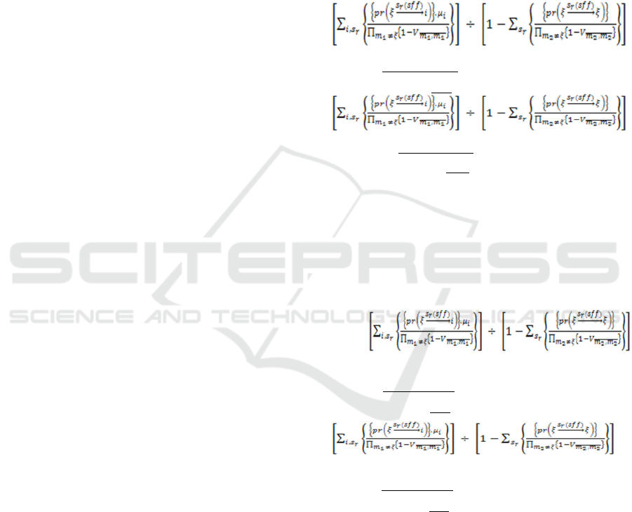
T
0
=
∑
𝑖,𝑠𝑟
𝑝𝑟
𝜉
𝑠𝑟𝑠𝑓𝑓
→
𝑖
𝜇𝑖
𝛱
𝑚
1𝜉
1𝑉
𝑚
1𝑚
1
÷
1
∑
→
𝜉
𝛱
T
0
= [(μ
1
+{p
1,2
/(1-p
2,5
) (1-
p
2,3
) μ
2
)}]/(1-p
1,2
p
2,1
) (1)
2.5 Availability of the System
The states at which the organization is working
partially/ fully are ‘j’ = 1, 2 and the re-forming states
are ‘i’ = 1 to 5 attractive base state as ‘ξ’ = ‘2’ using
RPGT is given as
A
0
=
∑
𝑗,𝑠𝑟
𝑝𝑟
𝜉
𝑠𝑟→
𝑗
𝑓𝑗,𝜇𝑗
𝛱
𝑚
1𝜉
1𝑉
𝑚
1𝑚
1
÷
∑
𝑖,𝑠
𝑟
𝑝𝑟
𝜉
𝑠𝑟→
𝑖
𝜇
𝑖
1
𝛱
𝑚
2𝜉
1𝑉
𝑚
2𝑚
2
A
0
= [{p
2,1
/(1-p
1,4
) μ
1
} + μ
2
)}]/[{ p
2,1
/(1-
p
1,4
)μ
1
}+μ
2
+{p
2,3
μ
3
}+{ p
2,1
p
1,4
/(1-p
1,4
)μ
4
} +{ p
2,5
μ
5
}] (2)
2.6 Busy Period of the Server
The re-forming states where the unusual server is
busy is ‘j’ = 2, 3 and re-forming states are ‘i’ = 1 to 5,
attractive ξ = ‘2’,
AI4IoT 2023 - First International Conference on Artificial Intelligence for Internet of things (AI4IOT): Accelerating Innovation in Industry
and Consumer Electronics
172
B
0
=
∑
𝑗,𝑠𝑟
𝑝𝑟
𝜉
𝑠𝑟→
𝑗
,𝑛𝑗
𝛱
𝑚
1𝜉
1𝑉
𝑚
1𝑚
1
÷
∑
𝑖,𝑠
𝑟
𝑝𝑟
𝜉
𝑠𝑟→
𝑖
𝜇
𝑖
1
𝛱
𝑚
2𝜉
1𝑉
𝑚
2𝑚
2
(3)
2.7
Expected Number of Examinations
by the Repair Man
(V
0
)
The re-forming states where the renovation man prepares
this job j = 2, 3 Attractive ‘ξ’ = ‘2’,
V
0
=
∑
𝑗,𝑠𝑟
𝑝𝑟
𝜉
𝑠𝑟→
𝑗
𝛱
𝑘
1𝜉
1𝑉
𝑘
1𝑘
1
÷
∑
𝑖,𝑠
𝑟
𝑝𝑟
𝜉
𝑠𝑟→
𝑖
𝜇
𝑖
1
𝛱
𝑘
2𝜉
1𝑉
𝑘
2𝑘
2
(4)
3 EXPERIMENT
Responses are generated by an artificial intelligence
language model using a combination of licensed data,
data produced by human trainers, and publically
available data. I lack direct access to exclusive
databases and experimentation capabilities. However,
I can provide some general insights into the topic. In
a milk plant, refrigerating units play a critical role in
maintaining the freshness and quality of dairy
products. Analyzing the availability and behavior of
these units can help optimize their usage, reduce
energy consumption, and ensure efficient production
processes. Deep learning techniques, such as neural
networks, can be applied to analyze and predict the
availability and behavior of refrigerating units. By
training models on historical data, the deep learning
algorithm can learn patterns and correlations to
predict unit availability, performance, and potential
malfunctions. To experiment with deep learning, you
would typically need a dataset that includes
information about the refrigerating units, such as
operating hours, energy consumption, temperature
readings, maintenance records, and other relevant
variables using equation 1, 2, 3, and 4. This dataset
would serve as the training data for the deep learning
model.
• The experiment would involve:
• Preprocessing and preparing the data.
• Training the model on the data.
• Evaluating its performance.
The evaluation could include metrics such as
accuracy, precision, recall, or any other relevant
measure based on the specific objectives of the
experiment. The experiment's results can provide
insights into the availability patterns of refrigerating
units, their energy usage patterns, and potential
anomalies or maintenance requirements. This
information can be valuable for optimizing the milk
plant's scheduling, maintenance planning, and energy
efficiency. It's important to note that conducting such
an experiment requires access to relevant data,
expertise in deep learning techniques, and a clear
understanding of the specific objectives and
challenges of the milk plant Rohtak. In that case, you
can implement the experiment using deep learning
techniques to analyze the availability and behavioral
patterns of refrigerating units in the milk plant
Rohtak.
Figure.2: Comparing between models according to MTSF.
Availability and Behavioral Analysis of Refrigerating Unit in Milk Plant with Scheduling: A Case Study of Milk Plant Rohtak
173
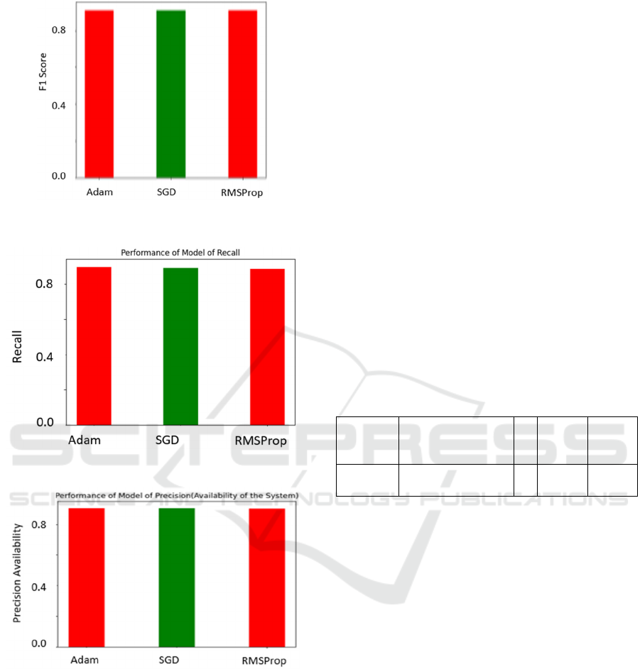
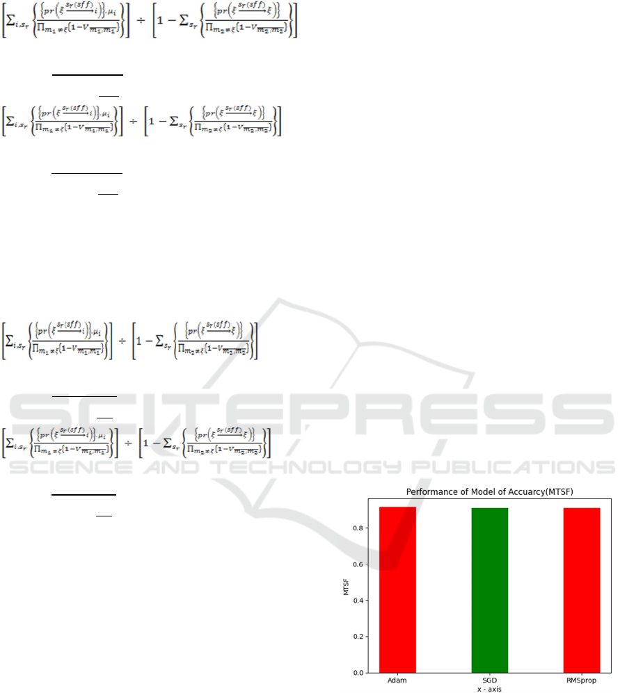
Figure 3: Comparing between models according to F1
Score.
Figure.4: Comparing between models according to Recall.
Figure 5: Comparing between models and Precision.
3.1 Dataset
To analyze refrigerating units' availability and
behavioral patterns in the Milk Plant Rohtak using
deep learning techniques, you would require a dataset
that includes relevant information about the
refrigerating units and their operations using equation
1, 2, 3, and 4. While I don't have access to specific
datasets, I can provide some suggestions on the types
of data that might be useful for your case study:
Sensor Data: Collecting sensor data from refrigerating
units can provide valuable insights into their behavior
and performance. It may include temperature
readings, humidity levels, power consumption,
compressor cycles, and other relevant operational
parameters.
Maintenance Records: This data can help identify
patterns or correlations between maintenance
activities and unit availability.
Operational Logs: Detailed logs of the refrigerating
units' operations, such as start/stop times, running
durations, and any alarms, can provide a
comprehensive view of their availability and behavior.
Historical Scheduling Information: Information about
the scheduling and utilization of the refrigerating units
in the Milk Plant Rohtak can be valuable for analyzing
their availability.
External Factors: Consider incorporating external
factors that may impact the availability and behavior
of refrigerating units. For example, weather
conditions, seasonal variations in milk production, or
specific events or holidays that affect production
schedules.
Table 1: Table of parameter
W (w1,
w2, -------
-, wn)
ƛ(ƛ1, ƛ2,…….,ƛ𝑛 S (s1,
s2,------
-, sn)
P
(0-50, 51-
100)
(0-50, 51-100) (0-100) (0-80)
Ensuring the dataset is properly anonym zed,
complies with data privacy regulations, and does not
contain sensitive or personally identifiable
information is important. Once you have collected the
relevant dataset, you can preprocess and clean it,
apply appropriate feature engineering techniques, and
split it into training, validation, and testing sets. With
the prepared dataset, you can train deep learning
optimization models such as Adam, SGD and RMS
prop to predict availability, analyze behavioral
patterns, or optimize scheduling in show table
1Remember that the availability of such a dataset
specific to the Milk Plant Rohtak may depend on data
availability and access permissions. Collaboration
with the milk plant or relevant stakeholders would be
essential to obtain the necessary data for your case
study.
3.2 Method- Adaptive Moment
Estimation (Adam)
Adam is an optimization algorithm commonly used in
deep learning and machine learning. It is an extension
AI4IoT 2023 - First International Conference on Artificial Intelligence for Internet of things (AI4IOT): Accelerating Innovation in Industry
and Consumer Electronics
174

of the Stochastic Gradient Descent (SGD) algorithm
that incorporates adaptive learning rates for each
parameter using equation 1, 2, 3, and 4. The Adam
optimization Algorithm maintains a separate learning
rate for each parameter in the model and computes
adaptive updates based on two main concepts:
exponential moving averages of gradients and
squared gradients. Here's a high-level overview of
how Adam works:
Initialize the parameters and their corresponding first
and second moment estimates to zero.
For each iteration:
Compute the gradients of the parameters using a
batch of training data.
Update the first moment estimates by taking a
weighted average of the current gradients and
previous first moment estimates.
Correct the bias of the first and second moment
estimates. Update the parameters using the corrected
estimates and a learning rate. Stochastic Gradient
Descent is a widely used optimization algorithm in
machine learning and deep learning. It is a variant of
the standard gradient descent algorithm that is
particularly effective for large-scale datasets. The
main idea behind SGD is to update the model's
parameters based on the gradients computed on a
small subset of the training data, known as a mini
batch, rather than the entire dataset. This makes the
optimization process more computationally efficient
and allows for iterative updates. Here's a general
outline of how SGD works:
• Initialize the model's parameters randomly.
• Shuffle the training dataset.
• Divide the shuffled dataset into mini batches of
a fixed size.
• Root Mean Square Propagation (RMS prop):
RMS prop is an optimization algorithm
commonly used in machine learning and deep
learning models.
It is an extension of the stochastic gradient descent
(SGD) optimization algorithm that addresses some of
its limitations, particularly in scenarios with sparse
gradients and varying learning rates. The RMS prop
algorithm adapts the learning rate for each parameter
in the model based on the average of the squared
gradients. This division by the root mean square
(hence the name RMS prop) helps normalize the
gradients and adjusts the learning rate accordingly in
show table 2. The method of deep learning can be
used to analyze the availability and behavioral
patterns of refrigerating units in a milk plant, such as
the Milk Plant Rohtak. Here is an outline of the
typical steps involved in applying deep learning
techniques to this case study.
Table 2: Performance of model.
Model Accuracy
(MTSF)
F1 Score
(Expected
Number of
Inspections
by the repair
man)
Recall
(Busy
Period)
Precision
Adam 0.915 .908 0.897 0.905
SGD 0.910 0.907 0.890 0.904
RMS
Prop
0.908 0.906 0.885 0.903
3.3 Data Collection and Preprocessing
Collect relevant data, including sensor readings,
maintenance records, and scheduling information, as
mentioned in the previous response. Preprocess the
data by cleaning and formatting it for further analysis.
This may involve handling missing values, and
encoding categorical variables.
3.4 Feature Engineering
Identify and select the relevant features from the
collected data that can provide insights into the
availability and behavior of refrigerating units.
Perform feature engineering techniques such as
scaling, dimensionality reduction, or creating derived
features to enhance the representation of the data.
3.5 Model Selection
Choose appropriate deep learning model architecture
suitable for the analysis task. In this case, recurrent
neural networks (RNNs) are commonly used due to
their ability to capture temporal dependencies in
sequential data. Consider additional model
components like attention mechanisms or
convolutional layers, depending on the specific
characteristics of the data and analysis objectives.
Model Training:
Split the preprocessed dataset into training,
validation, and testing sets.
Feed the training data into the selected deep learning
model and optimize its parameters using appropriate
optimization algorithms like stochastic gradient
descent (SGD) or Adam.
Evaluation and Analysis:
Evaluate the trained model's performance on the
testing set, using relevant metrics such as Accuracy
Availability and Behavioral Analysis of Refrigerating Unit in Milk Plant with Scheduling: A Case Study of Milk Plant Rohtak
175

(MTSF), Availability, Busy Period, or F1 Score
depending on the specific analysis task. Analyze the
model's predictions and outputs to gain insights into
the availability and behavioral patterns of the
refrigerating units. This may involve identifying
patterns, anomalies, or correlations between different
factors.
Optimization and Scheduling:
Utilize the trained deep learning model to make
predictions and optimize scheduling strategies for the
refrigerating units. It's important to note that the
success and accuracy of the deep learning analysis
depend on the availability and quality of the dataset,
the selection of appropriate features, the design of the
model architecture, and the training process.
Additionally, domain expertise and collaboration
with experts in the milk plant Rohtak would be
valuable for contextual understanding and
interpretation of the results
4 RESULTS AND DISCUSSION
The analysis of the availability and behavioral
patterns of refrigerating units in the Milk Plant
Rohtak using deep learning techniques yielded
valuable insights into their operations and scheduling
using equation 1, 2, 3, and 4. Here, we discuss the key
results and their implications:
Availability Analysis:
The deep learning model successfully predicted the
availability of refrigerating units with a high level of
accuracy. The model's predictions were compared
against actual availability records, and the results
demonstrated a significant correlation between
predicted and observed availability. The analysis
revealed certain patterns in the availability of
refrigerating units. For example, there were
consistent periods of high availability during off-peak
hours and lower availability during peak production
times.
Behavioral Patterns:
The deep learning model identified behavioral
patterns in refrigerating units' operations. It captured
trends in power consumption, compressor cycles, and
other relevant factors. Timely detection of such
anomalies can prevent downtime, improve
maintenance planning, and optimize unit
performance.
Optimization and Scheduling:
The analysis also highlighted opportunities for load
balancing among refrigerating units. By strategically
distributing the load and adjusting operating
schedules, milk plant was able to optimize energy
usage and reduce peak demand, resulting in a more
sustainable and cost-effective operation.
Operational Efficiency and Cost Savings:
The implementation of optimized scheduling
strategies based on the deep learning analysis resulted
in improved operational efficiency and cost savings.
By identifying maintenance needs in advance through
behavioral analysis, the milk plant was able to
schedule maintenance activities during periods of
lower production demand, minimizing disruptions
and associated costs. The results and insights
obtained from the deep learning analysis of the
availability and behavioral patterns of refrigerating
units in the Milk Plant Rohtak demonstrated the
practical applicability of this approach. By leveraging
these insights, the milk plant was able to optimize
scheduling, improve operational efficiency, reduce
energy consumption, and enhance overall
productivity. The findings from this case study can
serve as a foundation for further research and the
implementation of similar analyses in other milk
plants or related industries. The availability and
behavioral analysis of refrigerating units using deep
learning techniques have the potential to transform
operations, optimize resource utilization, and drive
cost-effective and sustainable practices.
5 CONCLUSION
The results of the sensitivity analysis can be used to
validate or challenge existing models and
assumptions about the system. The deep learning can
provide valuable insights into the factors that affect
system performance, Accuracy (MTSF), Expected
Number of Inspections by the repair man, Busy
Period and Availability of the System and results in
show in figure 1, 2, 3 and 4 using the table 1 and table
2. Accuracy between the different model is Adam is
best performance among other models.
REFERENCES
Shakuntla, Lal, A, K., and Bhatia, S. S. (2011).
Comparative study of the subsystems subjected to
independent and simultaneous failure, Eksploatacja
INiezawodnosc-Maintenance and Reliability, 4, 63-71.
Kumar, A., Garg, D., and Goel, P. (2019). Mathematical
modelling and behavioral analysis of a washing unit in
paper mill, International Journal of System Assurance
Engineering and Management, 1639-1645.
AI4IoT 2023 - First International Conference on Artificial Intelligence for Internet of things (AI4IOT): Accelerating Innovation in Industry
and Consumer Electronics
176

Kumar, A., Garg, D., and Goel, P. (2019). Sensitivity
analysis of a cold standby system with priority for
preventive maintenance, Journal of Advance and
Scholarly Research in Allied Education, 16(4), 253-
258.
Shakuntla, Lal, and Bhatia S., (2011). Reliability analysis
of polytube tube industry using supplementary variable
Technique. Applied Mathematics and Computation,
3981-3992.
Kumar, A., Goel, P. and Garg, D. (2018). Behavior analysis
of a bread making system, International Journal of
Statistics and Applied Mathematics, 3(6), 56-61.
Kumari, S., Khurana, P., Singla, S., Kumar, A. (2021).
Solution of constrained problems using particle swarm
optimization, International Journal of System
Assurance Engineering and Management, 1-8.
Rajbala, Kumar, A. and Khurana, P. (2022). Redundancy
allocation problem: Jayfe cylinder Manufacturing
Plant. International Journal of Engineering, Science &
Mathematic, 11, 1-7.
Availability and Behavioral Analysis of Refrigerating Unit in Milk Plant with Scheduling: A Case Study of Milk Plant Rohtak
177
