
Reliability and Availability Analysis of Non-Markovian Single Unit
Redundant System with Server Failure
Sanju Kumari
1
,
Sangeeta Malik
1
and Jai Bhagwan
2
1
Department of Mathematics, Baba Mastnath University Asthal Bohar, Rohtak, Haryana, India
2
Department of Mathematics, Govt P. G. Nehru College, Jhajjar, Haryana, India
Keywords: Non-Markovian, Availability, MTSF.
Abstract: In this paper reliability and availability modeling of a single unit having identical subunits in parallel with
cold standby redundant unit non- Markovian system having server which may also fail using Regenerative
Point Graphical Technique (RPGT) is developed aimed at deriving system parameters of the system followed
by analysis. A system can involve of several units and specific units obligate great importance in the proper
functioning of a system. Repairing of failed unit(s), is carried out, when it is completely failed by the server
(S) and is available in the system thereafter, who is to replace the failed units and responsible for the optimum
operation/functioning and maintenance of the system, which may also fail and is repaired by a specialist on
call is discussed and repair of unit A is imperfect and that of cold standby unit B is perfect, upon failure of
server or its non-availability a specialist is called for the operation and maintenance of system. Priority order
in repair is S>B>A. Various path probabilities, mean sojourn time and system behavior is discussed by
drawing tables for increasing failure/repair rates and graphs.
1 INTRODUCTION
Non-Markovian Process: Any process that depends
on all the past states is a non-Markovian process,
which implies that the memory of the previously
visited sites changes the distribution.
Here, for the reliability and availability modelling
of a single unit system A by a cold standby unit B is
considered, in which unit A have identical subunits in
parallel, hence if one/more of its subunit(s) flop, then
the system workings in reduced capacity and if the
number of subunits failure is superior than a
predefined number, then the system is in the failed
state, then the standby redundant unit B is replaced
with failed unit A, further upon failure of the standby
unit B, causes the whole arrangement to be in failed
state. A single server who is called in only when the
unit A is in failed state, and is available in the system
thereafter, who is to replace the failed units and
responsible for the proper operation/functioning and
maintenance of the system, which may also fail and
is repaired by a specialist on call is discussed. Repair
of failed unit A is imperfect. So, here the duration
during which the system stays in initial state S0,
depicts reliability of the system and availability is
evaluated from the subsequent states in which system
works in reduced states. Priority order in repair is
S>B>A. Taking failure/repair rates of units’
exponential, independent differently distributed and
enchanting into deliberation various transition
likelihoods, a state transition diagram of the
organization is industrialized to find different levels
of primary, secondary and tertiary circuits. Problem
is attempted using RPGT to model system
parameters. Various path probabilities mean sojourn
time and system behavior is discussed by drawing
tables for increasing failure/repair rates and graphs.
(Devi and Garg 2022) discussed the three algorithms
specifically HA, COGA and HGAPSO are applied to
solve RAP. Present paper carriages a comprehensive
literature review to classify, evaluate and intercept the
standing studies related to the RAP (Devi et al. 2023)
behavior of a bread plant was examined by (Kumar et
al. 2018). To do a sensitivity analysis on a cold
standby framework made up of two identical units
with server failure and prioritized for preventative
maintenance, (Kumar et al. 2019) used RPGT, two
halves make up the paper, one of which is in use and
the other of which is in cold standby mode. (Kumar
et al. 2019) investigated mathematical formulation
and behavior study of a paper mill washing unit, PSO
was used by (Kumari et al. 2021) to research limited
Kumari, S., Malik, S. and Bhagwan, J.
Reliability and Availability Analysis of Non-Markovian Single Unit Redundant System with Server Failure.
DOI: 10.5220/0012609900003739
Paper published under CC license (CC BY-NC-ND 4.0)
In Proceedings of the 1st International Conference on Artificial Intelligence for Internet of Things: Accelerating Innovation in Industry and Consumer Electronics (AI4IoT 2023), pages 571-577
ISBN: 978-989-758-661-3
Proceedings Copyright © 2024 by SCITEPRESS – Science and Technology Publications, Lda.
571
situations. Using a heuristic approach, (Rajbala et al.
2022) investigated the redundancy allocation
problem in the cylinder manufacturing plant.
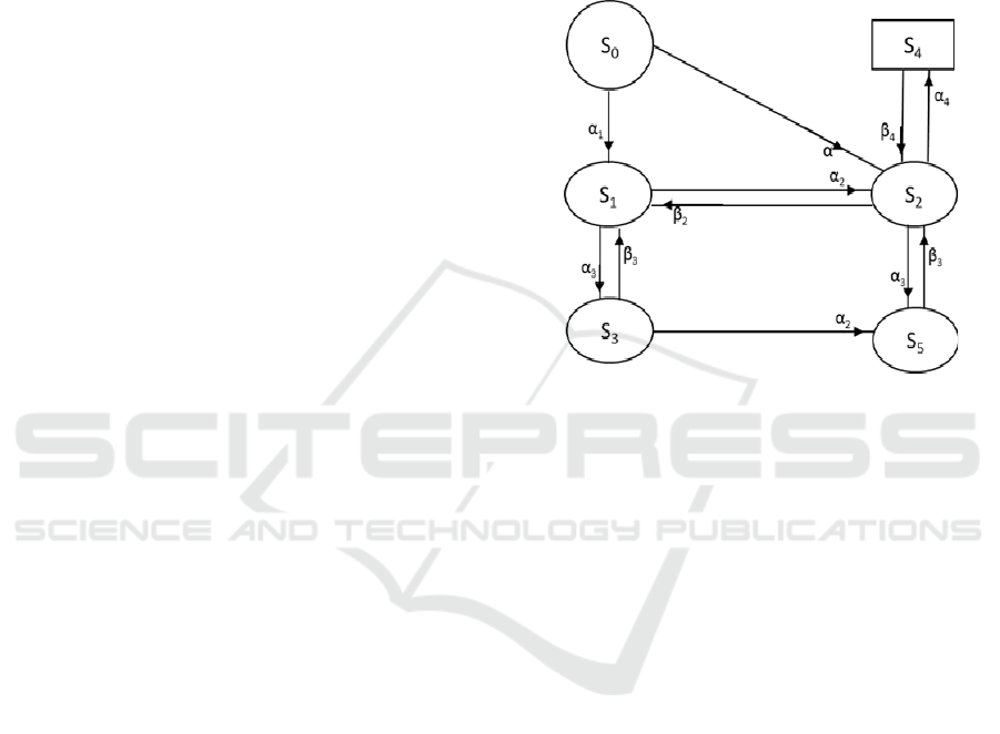
Model Description. Initially, system is in full
capacity working state S0[A(B)S], from which if the
unit A fails directly with transition rate α, then failed
unit A is replaced with standby unit B with the help
of server S, then the system enters the reduced state
S2[aBS] from which unit A is repaired imperfectly
with transition rate β2, then the system enters the state
S1[̅(B)S] as the repair of unit A is imperfect and if
one/more subcomponents of unit A fail in state
S0[ABS] with transition rate α1, i.e., there is partial
failure in unit A, then the system enters the state
S1[̅(B)S], while in state S1[̅BS] if server fails
whose transition rate is α3 then the system enters the
failed state S3[̅Bs] from which server is repaired on
priority at transition rate β3 and the system again
reaches the state S1, if in state S1 the reduced unit ̅
further fails to complete failure mode ‘a’ with
transition rate α2, then the unit B is switched in with
the help of the server and system enters the state
S2[aBS], if in state S2, if the unit B fails with
transition rate α4, then the organization enters the
failed state S4[abS], upon its restoration by the server
it re-joins the state S2, from which state if the server
S fails with transition rate α3, then the system enters
the failed state S5[aBs] as failed switch is unable to
keep the system in operation, from which the server
is given priority in repair with rate β3, so after repair
the system enters the state S2[aBS].
2 ASSUMPTIONS AND
NOTATIONS
1. There is one repairman whose availability is 24/7
after joining the system and specialist server is called
on need basis.
2. The distributions of disappointment and repair
times are constant, different and statistically
independent.
3. Nothing can flop when the organization is in failed
state.
α: Direct continuous failure rate of main unit A to ɑ
α1: Failure rate of unit A to reduced state ̅.
α2/ β2: Failure/repair rate of unit A since
reduced/failed state
α3/ β3: Failure/repair rate of server S
α4/ β4: Failure/repair rate of standby unit B.
A/̅/a: Unit in complete capacity operational /
reduced / failed state. B/(B)/b: Unit B is good online
/cold standby /failed mode.
S/s: server in good/failed state
3 TRANSITION DIAGRAM
DESCRIPTION
Figure 1: Transition Diagram.
Where various states are as under,
S
0
= A(B)S; S
1
= A ̅(B)S; S
2
= aBS; S
3
= A ̅(B)s;
S
4
= abS; S
5
= a(B)s
3.1 Probability Density Function (q
i,j
(t)
)
0,1
() = 1
(+1 );
0,2
() =
(+1 );
1,2
() = 2
(2 +3 );
1
,
3
() = 3
(2
+3 );
2
,
4
() = 4
(
2
+3+ 4 );
3
,
1
() =
3
(3 +2 );
3
,
5
() = 2
(3 +2 )
4
,
2
() = 4
4
;
5
,
2
() = 3
3
P
ij
= q*
i,j
(t)
0,1
= α
1
/(α+α
1
);
0,2
= α/(α+α
1
);
1,2
= α
2
/(α
2
+α
3
)
1,3
= α
3
/(α
2
+α
3
);
2,1
=
2
/(β
2
+α
3
+ α
4
);
2,4
=
α
4
/(β
2
+α
3
+ α
4
);
2,5
= α
3
/(β
2
+α
3
+ α
4
);
3,1
= β
2
/(β
3
+α
2
);
3,5
= α
2
/(β
3
+α
2
);
4,2
= 1;
5,2
= 1
3.2 Probability Density Functions R
i
(t)
and Mean Sojourn times µ
i
=R
i
*(0)
0
(t)=
(+1 );
1
(t)=
(2 +3 )
AI4IoT 2023 - First International Conference on Artificial Intelligence for Internet of things (AI4IOT): Accelerating Innovation in Industry
and Consumer Electronics
572
2
(t)=
(
2
+3+α
4
);
3
(t)=
(3+2 )
4
(t)=
4
;
5
(t)=
3
Value of the Parameter µ
i
giving Mean Sojourn
Times
µ
0
= 1/(α+α
1
); µ
1
= 1/(α
2
+α
3
) ; µ
2
=
1/(
2
+3+α
4
); µ
3
= 1/(β
3
+α
2
) µ
4
= (1/β
4
); µ
5
= (1/β
3
)
3.3 Evaluation of Parameters
Applying RPGT, path probabilities of reachable
states from initial state to different vertices are as
under
V
2
,
0
= 0 ; V
2
,
1
= [β2/(β2+α3+ α4)/{1- α3/(α2+α3)
β2/(β3+α2)}]; V
2
,
2
= 1 (verified); V
2
,3 = [β2/(β2+α3+
α4 α3/(α2+α3))/{1- α3/(α2+α3) β2/(β3+α2)]; V
2
,
4
=
α4/(β2+α3+ α4); V
2
,
5
= α3/(β2+α3+ α4)
3.3.1 MTSF (T
0
)
States to which organization can transit (from initial
state 0), before transiting/staying to any abortive state
are j = 0, 1, 5 2, 3, attractive initial state as ‘ξ’ = ‘2’.
Spread on RPGT, MTSF remains given as
T
0
=
÷
(1)
3.3.2 Availability of the System
States at where organization is accessible are j = 0, 1,
2, 3, 5 and attractive base state as ‘ξ’ = ‘2’ system
accessibility is specified by
A
0
=
÷
(2)
=
3.3.3 Busy Period of the Server
The recreating states where the server is busy while
liability repairs are ‘j’ = 1 to 5 and the re-forming
states remain ‘i’ = 0 to 2. Attractive ‘ξ’ = 2, the total
fraction of period aimed at which the attendant
remains busy is
B
0
=
÷
(3)
=
3.3.4 Expected Number of Examinations
by the Repair Man (V
0
)
The re-forming states where the waitperson visits a
fresh aimed at repair of organization stand ‘j’ = 1,2
and re-forming states stand ‘i’ = 1 to 11 aimed at ξ =
2,
V
0
=
÷
(4)
=
Reliability and Availability Analysis of Non-Markovian Single Unit Redundant System with Server Failure
573

4 EXPERIMENT
Performing a reliability and availability of non
markovian single unit redundant system with server
failure using deep learning requires several steps in
equation 1, 2, 3 and 4 to include for model to find
different parameter. Here is an example experiment
that you could perform:
● Collect data: Gather a dataset that contains
information on the input parameters and the
system's output. The input parameters could
include factors such as the system's design,
operating conditions, and maintenance
schedule. The output could include metrics
such as system availability, downtime, and
failure rate in table 1 and table 2.
● Preprocess data: Clean and preprocess the
dataset, splitting it into training, validation,
and test sets.
● Train the model: Use a deep learning
algorithm, such as a neural network, to model
the connection among the input parameters
and the output. Train the model by the training
set and validate it using the set of values in
table 1. You could use techniques such as early
stopping and regularization to prevent over
fitting.
● Appraise the model: After the model is
proficient, appraise its performance by means
of test set. Estimate metrics such as busy
period.
● Perform sensitivity analysis: Using the trained
model, vary the values of one parameter at a
time while keeping the others constant.
Record the effect on the system's output.
Repeat this process for each input parameter,
recording the impact of each parameter on the
system's output.
● Interpret results: Analyze the consequences of
the sensitivity examination to determine
which input parameters need the most
significant influence on the system's output.
You could use systems such as nose
importance and fractional dependence plots to
increase understandings into the mockup's
behavior.
4.1 Dataset
Sensitivity analysis is a way used to study how
variations in the input parameters of an organization
move the output. In the background of a reliability
and availability of non markovian single unit
redundant system can help determine which
parameters have the most significant impact on the
system's reliability. To perform sensitivity analysis
using deep learning, you would need a dataset that
contains information on the input parameters and the
system's output. The output could include metrics
such as system availability, Accuracy, and busy
period Once you have a dataset, you could use a deep
learning algorithm to model the relationship among
the input parameters and the production. One
approach could be to use a neural network, which can
learn complex relationships between inputs and
outputs. To perform sensitivity analysis using a
neural network, you could first train the network on
the dataset, using a portion of the data for training and
another portion for validation. Once the network is
trained, you could use it to make predictions on new
input data, varying the values of one parameter at a
time while keeping the others constant. By observing
how changes in each parameter affect the system's
output, you can determine which parameters have the
most significant impact on the system's reliability to
included dataset Table 1. Overall, sensitivity analysis
using deep learning can be an influential tool for
understanding the issues that pay to the reliability and
availability of non markovian single unit redundant
system. However, it requires a large and well-curated
dataset, as well as expertise in deep learning
techniques.
Table 1: Table of parameter.
W (w1,w2,---
--,wn)
(1,
S(s,s2,------
-sn)
P
(0-20,21-100)
(0-30,31-100)
(0-100)
(0-80)
5 RESULTS AND DISCUSSION
Reliability and availability of non markovian single
unit redundant system using deep learning typically
involves the following steps:
Data collection: Collect data on the input
parameters and output metrics of the system. The
input parameters could include factors such as the
system's design, operating conditions, and
maintenance schedule. The output metrics could
AI4IoT 2023 - First International Conference on Artificial Intelligence for Internet of things (AI4IOT): Accelerating Innovation in Industry
and Consumer Electronics
574

include measures such as system availability,
Accuracy, and busy period in show table 2 included.
Data preprocessing: Clean and preprocess the
data, splitting it into training, validation, and test sets.
Normalize the input variables to ensure that they are
on the same scale.
Model selection: Choose appropriate deep
learning optimization techniques (Adam, SGD, RMS
prop) for the sensitivity analysis. Some options
contain feed forward neural systems, convolutional
neural systems, and regular neural networks.
Consider influences such as the size of the dataset, the
difficulty of the input-output connection, and the
computational capitals existing.
Model training: Train the selected model on the
training data. Use techniques such as stochastic
gradient descent and back propagation to minimize
the bust time. Monitor the performance of the model
on the validation data, and adjust the hyper
parameters as needed.
Model evaluation: Assess the qualified model on
the test data. Calculate metrics such as mean absolute
bust time and mean squared error to assess the
model's performance of deep learning optimization in
show table 1 and table 2.
Table 2: Performance of model.
Model
Accuracy
(MTSF)
F1 Score
(Expected
Number of
serverby the
repair man)
Recall
(Busy
Period)
Precision
Adam
0.923
.9067
0.8012
0.9345
SGD
0.9123
0.9000
0.8123
0.9123
RMS prop
0.9012
0.8912
0.8103
0.9245
Sensitivity analysis: Use the trained model to
perform sensitivity analysis on the input parameters.
Vary the value of one input parameter at a time while
holding the others constant. Record the effect on the
output metric of interest. Repeat this process for each
participation parameter to determine the sensitivity of
the output metric to changes in each parameter.
Interpretation of results: Analyze the fallouts of
the sensitivity examination to identify which input
limits must the utmost impact on the output metric of
interest. Use practices such as article importance and
incomplete dependence plots to advance insights into
the association amid the input limits and output
metric.
Overall, performing reliability and availability of
non markovian single unit redundant system using
deep learning involves a combination of data
collection, preprocessing, model selection, training,
evaluation, and analysis.
It can be a commanding tool for understanding the
influences that underwrite to the reliability of the
system.
The results and discussion of a reliability and
availability of non markovian single unit redundant
system using deep learning will depend on the
specific system and dataset analysed. However, here
are some general insights that could be gained from
such an analysis:
Identification of critical system parameters: The
sensitivity analysis could reveal which input
parameters require the greatest effect on the output
metric of interest.
Understanding of the non-linear relationship
amongst input strictures and output metrics: The deep
learning model used in the analysis can capture non-
linear relationships amongst input restrictions and
output metrics, which could not be detected using
traditional statistical methods.
Validation of existing models and assumptions:
The results of the sensitivity analysis can be used to
validate or challenge existing models and
assumptions about the system.
Prediction of system behavior under different
scenarios: The deep learning model can be used to
predict system performance under different setups,
such as vagaries in operating conditions or
maintenance schedules.
Overall, sensitivity analysis of system parameters
of a reliability and availability of non markovian
single unit redundant system using deep learning can
provide valuable insights into the factors that affect
system performance, Accuracy (MTSF), Expected
Number of Check-ups by the repair man, Busy
Period and Availability of the System and results
in show in figure 2, 3, 4 and 5.
Accuracy between the different model is Adam is
best performance among them. And busy time of
Adam is better among them of model.
6 CONCLUSION
The results of the sensitivity analysis can be used to
validate or challenge existing models and
assumptions about the system. For example, the
analysis could show that a certain parameter has a
much greater impact on system performance than
previously thought. It can help optimize maintenance
strategies, improve system design, and reduce
downtime and maintenance costs.
Reliability and Availability Analysis of Non-Markovian Single Unit Redundant System with Server Failure
575
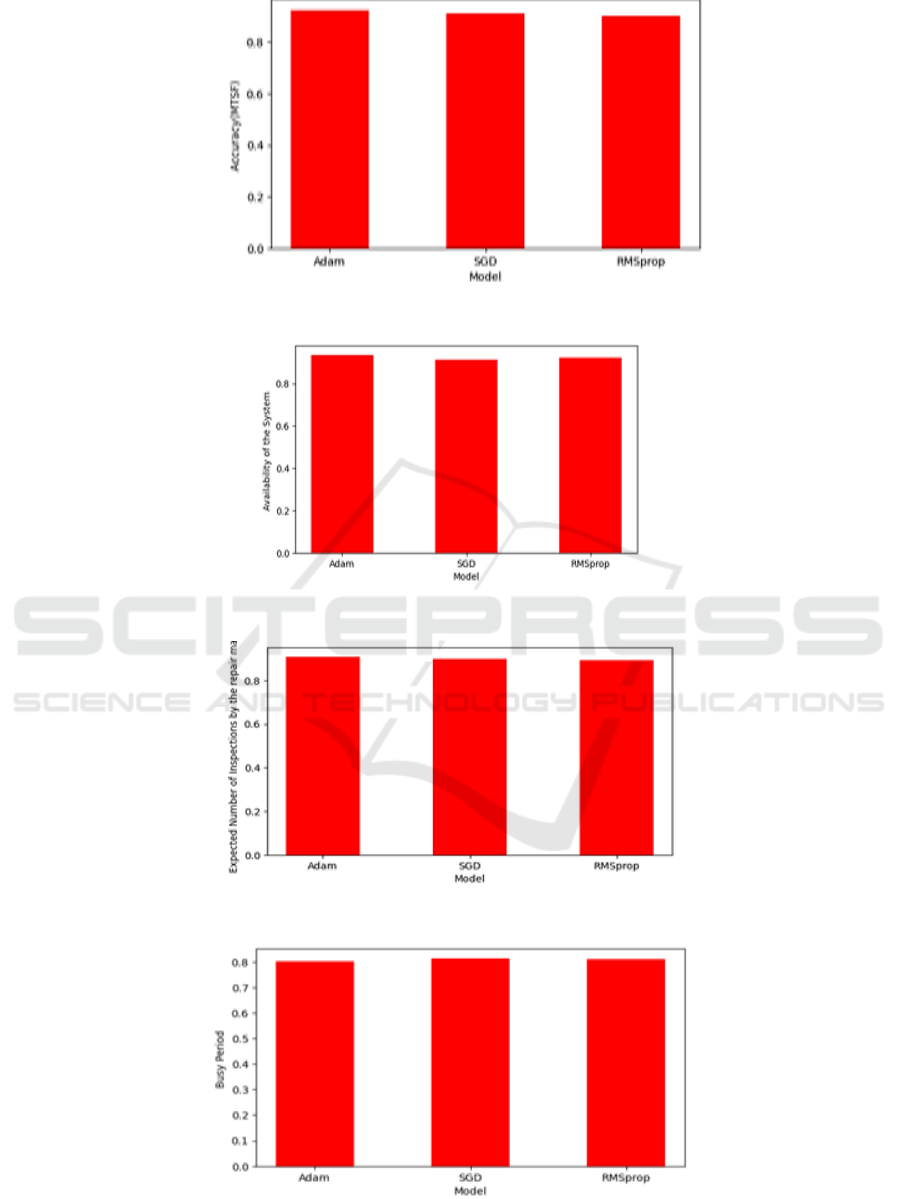
Figure 2: Comparison between Accuracy of models.
Figure 3: Comparison between Availability of model.
Figure 4: Comparison between Busy periods of models.
Figure 5: Comparison between models according to Expected Number of Examinations by the repair man.
AI4IoT 2023 - First International Conference on Artificial Intelligence for Internet of things (AI4IOT): Accelerating Innovation in Industry
and Consumer Electronics
576

REFERENCES
Devi, S., Garg, H. & Garg, D. (2023). A review of
redundancy allocation problem for two decades:
bibliometrics and future directions. Artif Intell Rev, 56,
7457–7548.
Kumar, A., Garg, D., and Goel, P. (2019). Mathematical
modelling and behavioral analysis of a washing unit in
paper mill, International Journal of System Assurance
Engineering and Management, 1(6), 1639-1645.
Kumar, A., Garg, D., and Goel, P. (2019). Sensitivity
analysis of a cold standby system with priority for
preventive maintenance, Journal of Advance and
Scholarly
Devi, S., Garg, D. (2020). Hybrid genetic and particle
swarm algorithm: redundancy allocation problem. Int J
Syst Assur Eng Manag 11, 313–319.
Kumar, A., Goel, P. and Garg, D. (2018). Behavior analysis
of a bread making system, International Journal of
Statistics and Applied Mathematics, 3(6),
Kumari, S., Khurana, P., Singla, S., Kumar, A. (2021).
Solution of constrained problems using particle swarm
optimization, International Journal of System
Assurance Engineering and Management, 1-8.
Rajbala, Kumar, A. and Khurana, P. (2022). Redundancy
allocation problem: Jayfe cylinder Manufacturing
Plant. International Journal of Engineering, Science &
Mathematic, 11(1), 1
Reliability and Availability Analysis of Non-Markovian Single Unit Redundant System with Server Failure
577
