Analysis and Forecast of Influencing Factors of House Price in Boston

Boyao Zhang

Department of Mathematics, The University of Manchester, Manchester, U.K.

Keywords: Correlation Analysis, Multiple Linear Regression, All-Subsets Regression, Random Forest Regression,

Variable Importance Plot.

Abstract: The cost of housing is a significant indicator of economic activity. Both buyers and developers of real estate

closely monitor fluctuations in home prices. As a result, developing an accurate housing price forecasting

model is critical for the financial market and people's livelihood. Boston dataset is used for data analysis in

this paper. Firstly, this paper conducted a correlation study using Pearson's r and created scatter plots

between each variable and the house price. In the multiple linear regression model, this study employed

techniques including outlier removal, collinearity, and variable transformation to optimize the model for a

more accurate prediction, finally getting an R-squared of 0.7927. In random forest model, this research finds

the optimal parameter value and then compares the importance of predictors using the indicators %IncMSE

and %IncNodePurity. Finally, this study determines that the random forest regression model is superior

through the investigation of the factors that influence home prices, and this paper also analyze the elements

that influence house prices and consider the shortcomings of this paper.

1 INTRODUCTION

Due to economic growth as well as non-economic

considerations including the caliber of schools, air

pollution levels, and distance from commercial hubs,

housing costs in major Chinese cities have been

continuously rising (Chen, 2023). To completely

comprehend the variables influencing house prices, a

multidimensional analysis is required. This study

examines the determining elements of housing costs,

including non-economic ones, utilizing reliable data

from 506 families in different Boston neighborhoods

(Harrison and Rubinfeld, 1978). The data is analyzed

using two different regression models, which can be

used as a guide for future studies on the factors

influencing housing costs in different Chinese cities.

Numerous specialists domestically and

internationally have conducted statistical analyses on

the factors influencing the cost of housing. For

instance, Chen Zekun and Cheng Xiaorong used the

gradient descent approach to perform regression

analysis on the data set, train the model to achieve

the fitting function, and then develop a housing price

prediction model (Chen and Cheng, 2020). Yin

Wenwen stated the coefficient function using a

verification methodology, and then used Boston

housing data to establish a variable coefficient model

with measurement errors, which adequately

explained the fluctuation trend of the median house

price. The verification approach can handle complex

error structure models while saving a significant

amount of money (Yin, 2018). Keren Horn, and

Mark Merante investigated the influence of Airbnb

on rental pricing, attempting to determine whether

changes in rental prices are related to a drop in

housing availability (Horn and Merante, 2017).

2 RESEARCH METHOD

2.1 Pearson’s Correlation Coefficient

It is a commonly used linear correlation metric. The

covariance between two vectors, normalized by the

product of their standard deviations, is how it is

defined (Makowski, et al, 2020). The coefficient

measures the tendency of two vector pairs to change

collectively above or below their mean, indicating

that the measurements for each pair are more likely

to fall on one side or the other of the average for that

pair.

2.2 Model Selection

A linear regression model with numerous explanatory

Zhang, B.

Analysis and Forecast of Inﬂuencing Factors of House Price in Boston.

DOI: 10.5220/0012797700003885

Paper published under CC license (CC BY-NC-ND 4.0)

In Proceedings of the 1st International Conference on Data Analysis and Machine Learning (DAML 2023), pages 107-113

ISBN: 978-989-758-705-4

107

variables is known as a multiple linear regression

model (Kumari and Yadav, 2018). This paper can

take into consideration the following linear

relationship:

y β



β



β



⋯β



ε (1)

y=MEDV(the median value of owner-occupied

homes) , x





,…,x



=factors affecting housing

prices. 𝛽



and 𝛽



,…𝛽



are intercept term and the

regression coefficient respectively, and ε is the error

term representing random errors that the model

cannot explain (Burton, 2021).

Random forest regression is an ensemble

learning-based algorithm that performs regression

tasks by building multiple decision trees and

integrating their predictions. A random forest

effectively lowers the danger of overfitting because

each decision tree is independent and trained on

randomly chosen subsamples. To obtain the final

regression result, the random forest weights or

averages the predictions of various decision trees 0

Qin and Song, 2021).

3 DATA ANALYSIS

Each of the 506 entries in the Boston housing data

provides aggregated information about 14 attributes

of dwellings in different Boston areas that were

collected in 1978 (Harrison and Rubinfeld, 1978).

The explanation of each variable is given in

following table 1:

Table 1: Factors affecting Boston house prices.

Variable

name

Variable interpretation

CRIM 𝑥



Criminal rate per capita by town.

ZN 𝑥



Residential use is permitted on lots

Lar

er than 25,000 s

uare feet.

INDUS 𝑥



Each town's percentage of non-retail

usinesses.

CHAS 𝑥



The dummy variable for Charles River

(= 1 is a river; =0 is not a river).

NOX 𝑥



Nitrogen oxides concentration

arts

er 10 million

)

RM 𝑥



Rooms available per home.

AGE 𝑥



Proportion of pre-1940 owner-occupied

housing units.

DIS 𝑥



Distance from five Boston job centers,

weighted.

RAD 𝑥



Accessibility score for radial highways.

TAX 𝑥



Property tax rate per $10,000 of full value.

PIRATIO

Town-specific student-teacher ratio.

𝑥



B 𝑥



1000𝐵𝑘  0.63



Where Bk is the

ercentage of blacks.

LSTAT 𝑥



Lower status of the population (percent).

MEDV y

The average cost of an owner-occupied

residence is $1000.

To examine the factors influencing the level of

house prices, this paper selects MEDV as my

response variable and the other 13 variables as

explanatory variables out of these 14.

3.1 Descriptive and Correlated

Analysis of Data

This paper uses R software for analysis. For each

variable, Table 2 displays the descriptive statistics.

Table 2: Descriptive Analysis of Explanatory Variables

CRIM ZN INDUS

n 506 506 506

NA 0 0 0

mean 3.61 11.4 11.1

Based on initial analysis, this study concludes

that the data do not contain any missing values.

Intuitively, these factors will affect the level of

housing prices in Boston in 1987. In order to further

build the model, this research then assesses the link

between the explanatory variable and the

corresponding variable using the scatter plot and

correlation coefficient plot.

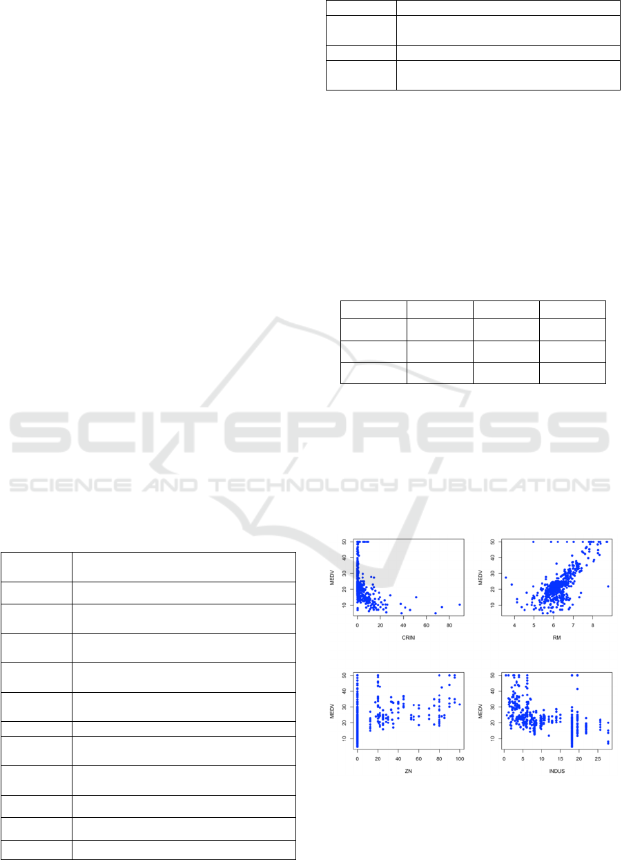
Figure 1: Scatter plot of each feature with MEDV (Picture

credit: Original).

Figure 1 above shows a positive correlation

between RM (the average number of rooms

DAML 2023 - International Conference on Data Analysis and Machine Learning

108

available) and MEDV, implying that the price of real

estate in the area will rise as the average number of

rooms per residence rises. Similarly, there is a

negative correlation between CRIM (for each person

criminal activity by town) and MEDV, which means

if the town's per capita crime rate rises, home values

will fall.

Figure 2: Plot of the correlation coefficient between

variables (Picture credit: Original).

As can be observed, there is a significant

association between LSTAT (the residents with a

lower socioeconomic status.), RM, PIRATIO (the

student-teacher ratios vary by town.), and MEDV,

with correlation values of -0.74, 0.70, and -0.51

accordingly. Moreover, the correlation coefficient

between the variable CHAS (the Charles River

imaginary variable) and the other factors is often in

the range of 0.1, demonstrating a minimal influence.

Because of this, this paper will ignore the variable

CHAS variable in further analysis.

3.2 Multiple Linear Regression

Model -- First Regression Analysis

The Boston data was manually divided into two sets:

the training set, which had 70% of the data, and the

test set, which contained 30% of the data. The first fit

to MEDV was performed using the remaining

variables based on training data. The regression

model is:

y  34.120254  0.09745X1 

0.031720X2  0.019334X3  15.542128X5 

4.001339X6  0.002983X7  1.283889X8 

0.300291X9  0.012381X10 

0.973398X11  0.009031X12  0.498439X13

The results show that p-value < 0.05, so the

author can reject the null hypothesis, which means

the regression equation is significant. A mediocre

fitting effect is shown by the fitting coefficient R-

squared of 0.742 and the adjusted R-squared of

0.733. The author then creates a fitting curve to

compare the true value of housing prices with the

expected value to assess the impact of the model of

multiple linear regression. As shown in figure 3:

Figure 3: The expected and true value fitting curve

(Picture credit: Original).

The extent of variation that can be explained by

the regression equation is indicated by the values of

R-squared, which are 0.719 and adjusted R-squared,

respectively, of 0.717. Since most of the sample data

points are grouped together around the regression

line, the model has a high goodness of fit, as can be

shown.

3.3 Model Optimization

First, this study uses the influence plot and outliers

test function in the car package to remove the

outliers, leverage values, and strong influence points

such as 366, 369,419 and so on (Kabacoff, 2011).

Next, this paper attempt to use the vif(fit) to identify

any data collinearity (Shrestha, 2020). Although the

VIF (variance inflation factor) of each variable is

very minor, multicollinearity is present because the

VIF values of NOX (the level of nitrogen oxides),

RAD(the use of circular highways), and TAX(the

full-value property-tax rate per$10000) are all higher

than 4. This paper can use the all-subsets regression

approach to screen out multicollinearity by filtering

variables on the boston data.

Figure 4 shows that CRIM, ZN (proportion of

residential land zoned), INDUS (The fraction of

acres used for non-retail businesses per village), and

RAD have little impact; hence, this study eliminate

these four variables. Finally, the scatter plot and

kernel density estimation curve are utilized to assess

the correlation between the variables and the MEDV

median house price (Zhang, 2018). Additionally,

Analysis and Forecast of Inﬂuencing Factors of House Price in Boston

109

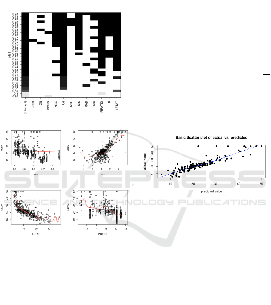
variable transformation is implemented to further

enhance the efficiency of the model.

Figure 4: Full subset regression (Picture credit: Original).

Figure 5: Scatter plot and kernel density estimation curve

(Picture credit: Original).

According to Figure 5, there may be a quadratic

correlation between RM and MEDV, a reciprocal

correlation between LSTAT and MEDV. It's not

immediately clear how much other factors and

MEDV are correlated. Therefore, this paper rebuilts

the regression model and added the two terms RM



and





to the original model.

3.4 Multiple Linear Regression

Model -- Final Regression Analysis

Below this paper carries out the fitting based on

training data (Table 3), only three random lines of

data are presented here:

Table 3: Coefficient of the regression Equation.

fitting Estimate Std.Error t value



𝑡



(Intercept) 100.23249 10.02214 10.00 < 2e-16

I(RM^2) 1.93103 0.21987 8.78 < 2e-16

I(1/LSTAT) 31.23698 5.57000 5.61 4.2e-08

The final regression model is obtained as:

y=100.2324913.58667𝑥



21.14899𝑥



0.001

49𝑥



0.83616𝑥



0.00261𝑥



0.66777𝑥



0.00

739𝑥



0.33427𝑥



1.93103𝑥





31.23698







Because of the test's p-value of 2e-16, the results

indicate that the null hypothesis can be rejected.

Fitting coefficient R-squared is 0.815 and adjusted R-

squared is 0.813. Similarly, this paper draws the

fitting curve of the genuine house price and the

forested house price to check the effect of model

optimization:

Figure 6: The expected and true value fitting curve

(Picture credit: Original).

Residual standard error is 4.46. R-squared is

0.787 and adjusted R-squared is 0.786. therefore,

compared to the initial regression model, the final

multiple linear regression model reflects an improved

goodness of fit for the clustered black points.

4 RANDOM FOREST

REGRESSION MODEL

4.1 Determine the Parameters of mtry

and ntree

This paper calls the random Forest function. First,

this study choose the best mtry for the model (He, Fu

and Liao, 2023). This paper adjusted the mtry

parameter value to 6 during this modeling procedure

since the traversal print result indicates that the

optimal value for % Var explained=0.8583 for

mtry=6. Next, this paper will find the model's ntree

value, which indicates how many decision trees were

DAML 2023 - International Conference on Data Analysis and Machine Learning

110

present at the time of modeling 0. To determine the

value of the ntree parameter, this paper created a

diagram below to illustrate the relationships between

the quantity of decision trees and the rate of model

inaccuracy.

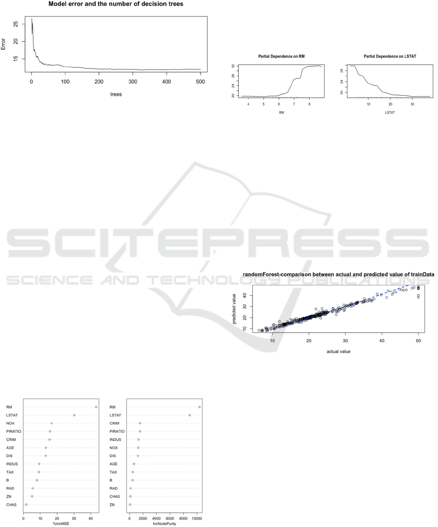
Figure 7: Relationship between model error rate and how

many decision trees (Picture credit: Original).

As shown in figure7, the error rate decreases if

the ntree value is 500. Therefore, this paper used

mtry=6 and ntree=500 as the model parameters, and

then the author trained the random forest model

based on the training set. The R-squared is 0.855 and

a mean squared residual of 11.76, indicating that the

regression result using the random forest model is

satisfactory. Next, this research will use the

metrics %IncMSE(the rise in Mean squared Error of

predictions) and %IncNodePurity(the mean decrease

accuracy) to assess the variable's significance.

4.2 Check the Importance of Predictor

Factors

Each predictor is given a random assignment, and the

increase in the model's prediction error is then noted

to determine the %IncMS (Liu et al, 2020). By

computing the summation of the residuals' squares to

compare the relative weights of the 13 variables,

IncNodePurity assesses the impact of each variable

on the heterogeneity of the observed values on the

classification tree's nodes. As seen in figure 8:

Figure 8: Variable Importance plot (Picture credit:

Original).

It can see from the two figures above that the

value of housing expenses are greatly influenced by

RM, indicating that the amount of rooms is the

primary factor determining the price of housing. The

partial dependence plot can be used to determine

whether there is a linear, monotonous, or complex

relationship between the predictor and the house

price. The following are examples of the partial

dependent plot for the association between RM,

LSTAT, and MEDV:

Figure 9: Partial dependence plot (Picture credit: Original).

As shown in figure 9, there is a strong linear

relationship between housing price and RM, while

LSTAT is negatively correlated with housing price,

which is the same as the above conclusion.

4.3 The Results of the Training Set

Prediction

This study tested the effect of the model by fitting the

regression model. Figure 10 depicts the training set's

prediction outcomes.

Figure 10: The results of the training set prediction

(Picture credit: Original).

Through fitting regression analysis of MEDV and the

predicted value of the training set, this study has the

value of R-squared multiple is 0.9765 and R-squared

adjusted is 0.9764, demonstrating the excellent data

training effect of the model of random forests.

4.4 The Anticipated Scores of the

Testing Set

This paper employs a trained random forest

regression model to produce predictions for the test

samples. The outcomes are as figure 11:

Analysis and Forecast of Inﬂuencing Factors of House Price in Boston

111

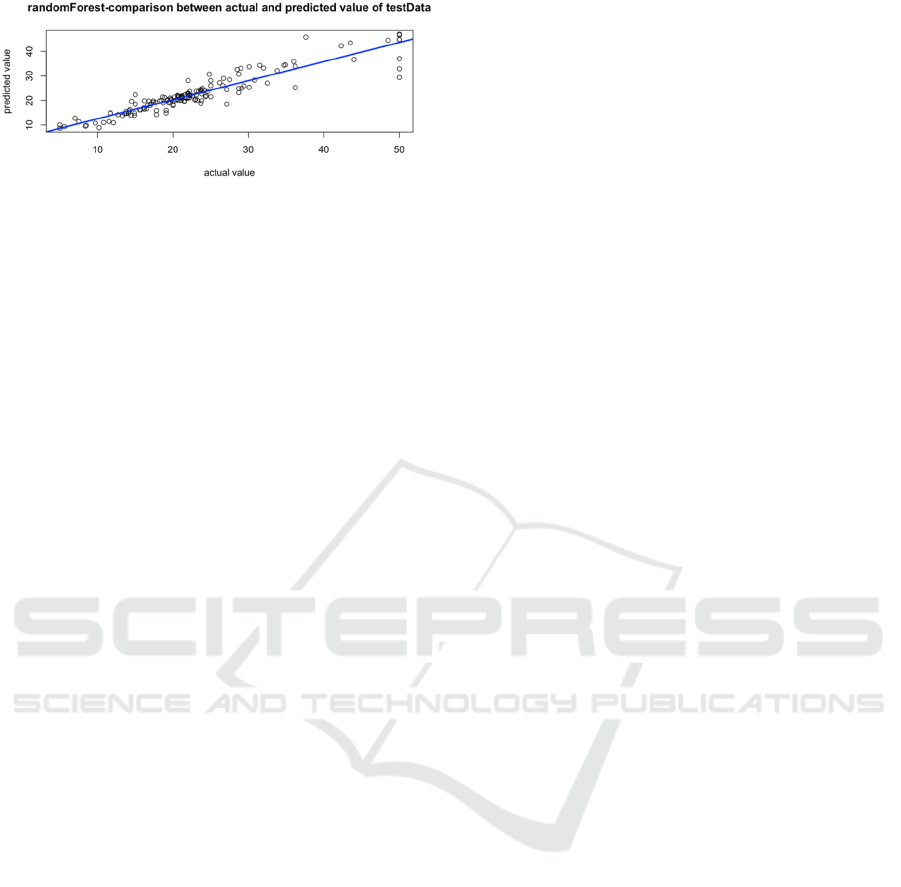
Figure 11: Testing set prediction outcomes (Picture credit:

Original).

This paper performed fitting regression analysis

on the median home price MEDV and the estimated

value of the test data, and the results showed that the

residual standard error is 3.033 and adjusted R-

squared value is 0.859. Many of the points are

clustered around the blue fitting line in the above

image, even though a tiny portion of the points are

dispersed across the fitting line, and the random-

forests model has a usually accurate prediction

consequence.

5 DISCUSSION

First, there are additional factors that affect the cost

of housing, such as size, kind, height, and condition.

Second, I eliminated variables and outliers that had

an impact on the model's fit during the data analysis

stage (Wang, Bah and Hammad, 2019).

6 CONCLUSION

6.1 Comparison between Different

Models

Residual standard error of multiple linear regression

prediction is 4.402 and the R-squared, a measure of

determination, is 0.7927. R-squared coefficient of

determination is 0.86, and the residual standard error

of the prediction from random forest regression is

3.033. The information demonstrates that the random

forest model is not only better than the linear

regression model in data fitting optimization, but also

has higher prediction accuracy than the linear

regression model.

6.2 Different Factors' Effects on Home

Prices

The regression coefficient and scatter plot of the

model show that the percent of people with fewer

socioeconomic status (LSTAT) and the sheer number

of rooms in the house (RM) have the biggest effects

on housing costs. In other words, the price of an area

increases exponentially as the count of rooms

increases. Likewise, when the population's share of

the lower class rises, average disposable income falls,

which in turn causes a decline in home values. The

price of a home decreases with increasing weighted

distance (DIS: locations of five Boston employment

centers. ) from Boston's five major neighborhoods,

but prices increase in areas with low nitric oxide

concentration (NOX), where there is greater housing

dispersal. The price of housing decreases when the

teacher-to-student ratio (PIRATIO) increases. High

property taxes have a negative effect on home prices,

but this effect is less pronounced in certain places.

6.3 Outlook

The above conclusions are from a macro point of

view, the conclusion is only general. If researchers

want to be specific to a particular house, they need to

analyze according to the actual local situation. At the

same time, due to time constraints, this study only

built and trained linear regression and random forest

models. It is hoped that more models will be added

for analysis and comparison in future studies, and the

optimal model will be selected for better prediction.

REFERENCES

SY Chen. "Study of the new juvenile housing safety in our

large metropolis——Take Shenzhen for example."

Shanghai Real Estate, vol.1, 2023, pp.41-45.

D.Harrison, and DL.Rubinfeld. "Hedonic housing prices

and the demand for clean air." Journal of

environmental economics and management, vol.5,

Mar.1978, pp.81-102.

ZK Chen, XR Cheng. "Regression analysis and prediction

of housing price based on gradient descent

algorithm. " Information Technology and

Informatization, vol.5, 2020, pp. 10-13.

WW Yin. "Research on verification methods of variable

coefficient error model of Boston housing data. "

Journal of Chongqing Technology and Business

University(Natural Science Edition), vol.3, 2018,

pp.26-29.

K.Horn, M.Merante. "Is Home Sharing Driving up Rents?

Evidence from Airbnb in Boston." Journal of

Housing Economics, vol.38, Dec.2017, pp.14-24.

D.Makowski, MS.Ben-Shachar, I.Patil, et al."Methods and

Algorithms for Correlation Analysis in R. " The

Journal of Open Source Software, vol.51, Jul.2020,

pp.2306.

DAML 2023 - International Conference on Data Analysis and Machine Learning

112

K.Kumari, S.Yadav. "Linear regression analysis study.

"Journal of the Practice of Cardiovascular Sciences,

vol.4, Jan.2018, pp.33.

AL.Burton. "OLS (Linear) Regression." The encyclopedia

of research methods in criminology and Criminal

Justice, vol.2, Aug.2021, pp.509-514.

ZX Yan, C Qin, G Song. "Random forest model stock

price prediction based on Pearson feature selection.

"Computer Engineering and Applications, vol.15,

Aug.2021, pp.57.

RI.Kabacoff. "R In Action: Data Analysis and Graphics

with R. " 1st. Shelter Island: Manning Publications

Co, Aug.2011.

N.Shrestha. "Detecting Multicollinearity in Regression

Analysis. " American Journal of Applied

Mathematics and Statistics, vol.8, Jun.2020, pp.39-

42.

JJ Zhang. "Evolution trend of resident income gap in five

northwest provinces: Analysis based on kernel

density estimation." Financial Theory and

Teaching,vol.3, 2018,pp.58-61.

WL He, LL Fu, JP Liao. "Study on pig price prediction

and regulation mechanism based on random forest

model." Prices Monthly, vol.1, 2023, pp.7.

J Liu, T Zhou, H Luo,et al. "Diverse Roles of Previous

Years' Water Conditions in Gross Primary

Productivity in China." Remote Sensing, vol.1,

2020.

Oritteropus. "[R] Partial dependence plot in randomForest

package (all flat responses)." [2023-08-25].

HZ Wang, M.Bah, M.Hammad. "Progress in Outlier

Detection Techniques: A Survey. " IEEE Access,

vol.7, Aug.2019, pp.107964-108000.

Analysis and Forecast of Inﬂuencing Factors of House Price in Boston

113