The Prediction of Carbon Dioxide Emissions and Parameter Analysis

Based on the LSTM

Yuxi Ji

Hang Zhou High School, Hangzhou, China

Keywords: Carbon Dioxide, Long Short-Term Memory, Prediction, LSTM Layers.

Abstract: The development of effective climate change mitigation methods and the understanding of the future effects

of climate change are made possible by accurate projections of carbon dioxide (CO2) emissions. This paper

uses the Long short-term memory (LSTM) model to increase the prediction accuracy of CO2 emissions.

Prediction issues can benefit from the use of the LSTM model. Specifically, this paper compares the Mean

squared error (MSE) value, representing the precision of CO2 emission prediction, for several LSTM layers

and epochs in great detail. This study is conducted on the U.S. Energy Information Administration's CO2

emissions from the coal power industry dataset. The experiment's findings show that increasing the number

of layers of LSTM can increase the prediction accuracy of CO2 emissions, while reducing the number of

layers would decrease that accuracy. Meanwhile, the number of epochs with the maximum prediction

accuracy of CO2 emissions under various epochs is 10, and there is no direct relationship between epochs and

prediction accuracy. This paper provides an efficient CO2 emission prediction model to provide a practical

method to mitigate the greenhouse effect by optimizing the parameters of the LSTM model.

1 INTRODUCTION

Given the "Paris Agreement" assurances to control the

status quo of global warming by regulating

greenhouse gas emissions, more individuals are now

beginning to pay attention to carbon emissions.

Climate extremes such as drought or storms, as well

as regional changes in temperature and precipitation

extremes, carbon dioxide (CO2) emissions, and other

factors could cause reductions in carbon stocks in

regional ecosystems, potentially offsetting the

anticipated increase in terrestrial carbon uptake and

having a significant impact on the carbon balance

(Seneviratne et al 2016 & Reichstein et al 2013). The

prediction of CO2 emissions is therefore necessary.

Large amounts of energy are used, and CO2 is

released as a result of the rapid expansion of industry.

Industrial companies can more easily accomplish

clean production, optimize energy structure, lower

production costs and carbon emissions, and exert

greater control over production conditions through

precise energy consumption and carbon emission

forecasts. Additionally, it manages the greenhouse

effect (Hu and Man 2023).

The calculation of CO2 emissions and the creation

of prediction models are current research areas for

numerous professionals and academics. A number of

models have been put forth, including the logarithmic

mean Divisia index (LMDI) method, the production

function theory, and a data-driven method (Ang 2005

& Wang et al 2019). Energy intensity is a significant

indicator for lowering CO2 emissions using the LMDI

approach, according to Zhang et al.'s analysis (Zhang

et al 2019). Models for predicting carbon emissions

rely on the direct or indirect transformation of energy

data to calculate emissions. Concerning the data-

driven method, machine learning techniques, which

depend on extrapolating energy usage patterns from

past data, are the main focus. To handle the time series

forecast of CO2 emissions, Abdel suggested an

artificial neural network model (ANN) that has four

inputs for global oil, natural gas, coal, and primary

energy consumption (Fang et al 2018). ANN, long

short-term memory (LSTM), etc. have all advanced

the study of CO2 emission prediction in recent years

(Tealab 2018 & Peng et al 2022).

The main objective of this study is to introduce the

deep learning technology of the LSTM framework to

improve the performance of CO2 emission prediction.

Specifically, first, LSTM networks are used to

evaluate CO2 emission forecasts. Second, LSTM

models are a development of recurrent neural

networks (RNN), and they provide a remedy for the

Ji, Y.

The Prediction of Carbon Dioxide Emissions and Parameter Analysis Based on the LSTM.

DOI: 10.5220/0012800100003885

Paper published under CC license (CC BY-NC-ND 4.0)

In Proceedings of the 1st International Conference on Data Analysis and Machine Learning (DAML 2023), pages 527-531

ISBN: 978-989-758-705-4

527

problem of RNN long-term dependency. The

application of LSTM for CO2 emission prediction is

appropriate since it is suitable for time series data

processing, forecasting, and classification (Rostamian

and Hara 2022). Third, the predictive performance of

the different models is analyzed and compared. This

study compares distinct LSTM layers and examines

the effectiveness of CO2 emission prediction across

multiple epochs. The experimental results

demonstrate that when the number of epochs is the

same, adding a layer of LSTM could boost CO2

emission forecast accuracy, while removing a layer

will reduce accuracy. Additionally, when the number

of LSTM layers is constant, there is a relationship

between the number of epochs and the prediction

accuracy of CO2 emissions, but it is neither

proportionate nor inversely proportional. In this

experiment, the number of epochs with the highest

prediction accuracy of CO2 emissions is 10. Finally,

this study can provide valuable insights into the field

of CO2 emission prediction. An accurate and efficient

CO2 emission prediction model can successfully

control CO2 emissions and slow down global

warming and other greenhouse effects.

2 METHODOLOGY

2.1 Dataset Description and

Preprocessing

The dataset used in this study, called Carbon

Emissions, is sourced from Kaggle (Dataset). The

Energy Information Administration's annual and

monthly CO2 emissions from the coal-electric power

sector are contained in the dataset. Millions of metric

tons of CO2 are the units. This experiment loads a

CSV file containing data on CO2 emissions before

data preprocessing. This experiment divides the

preprocessed data into a training set and a test set

based on whether the year is greater than or equal to

2015. It also only retains the year and value columns

and replaces any missing values with the mean value.

Then scale the data to make it suitable for the LSTM

model. Then the data is scaled to make it suitable for

the LSTM model while being normalized between a

range of -1 and 1.

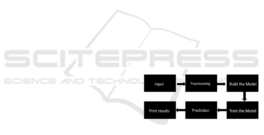
2.2 Proposed Approach

The main purpose of this study is to develop a model

that can accurately forecast future CO2 emission

levels while ensuring reliability and conciseness. The

foundation of this study lies in the utilization of LSTM

networks, which are well-suited for capturing

sequential patterns in time series data such as

historical CO2 emission data. To construct the model,

a systematic process, as illustrated in Fig. 1, is

followed. Initially, the input data undergoes

preprocessing to ensure its compatibility with the

LSTM architecture. This may involve steps like

normalization or scaling to facilitate optimal model

performance. Once the LSTM model is trained using

the preprocessed data, it is ready for predicting CO2

emissions on the test data. By feeding the test data into

the trained model, it generates forecasts that estimate

the future emission levels. These predictions are then

compared to the actual values using the Mean Squared

Error (MSE) metric.

The MSE quantifies the average squared

difference between the predicted and actual CO2

emission values, providing an objective measure of

the model's accuracy. A lower MSE indicates a more

precise and reliable forecasting model. By employing

LSTM networks and following a systematic approach,

this study aims to contribute to the development of an

effective model for forecasting future CO2 emission

levels. The utilization of the MSE metric ensures a

quantitative evaluation of the model's predictive

performance, thereby facilitating comparisons with

other forecasting methods and enabling policymakers

and stakeholders to make informed decisions

regarding carbon emissions mitigation strategies.

Figure 1: The pipeline of the model (Picture credit:

Original).

2.2.1 LSTM

A particular type of RNN called LSTM is able to gain

insight into the long-term dependencies of the

information gathered. Long-term retention of

memories is beneficial through the use of LSTM

since it has the capability to maintain an internal state.

This makes LSTM, therefore, extremely useful for

tasks like speech recognition, language modeling, and

predicting time series. The cell state and its

assortment of gates are what constitute the

fundamental concept of an LSTM. The internal

memory of the LSTM network incorporates the cell

state, which undergoes processing by input gates and

DAML 2023 - International Conference on Data Analysis and Machine Learning

528

forget gates. Sigmoid activations with compression

values between 0 and 1 can be observed in gates.

Since each of the numbers multiplied by 0 equals 0

and each and every number multiplied by 1

corresponds to the same value, the sigmoid activation

feature enables the network to determine which data

is crucial for storage and which data is of no

significance to throw away.

Three distinct gates in the LSTM are used to

control the information flow in the LSTM cells. The

first one is the input gate, which, as suggested by its

name, is in charge of taking input data. The input gate

will determine whether the input data should be added

to the cell state based on the sigmoid activation

function in accordance with the foregoing. The forget

gate is also in the position of selecting which data to

throw away. To choose which pieces of information to

keep track of, it also utilizes a sigmoid activation

function. The output gate is the final one. The LSTM

network's output is generated by the output gate via

the cell state. It creates an information vector that

depicts the current state of the system using a Tanh

activation process. In general, an LSTM network

evaluates new information, processes it, and then

stores it in the cell state. After passing through the

forget gate, where certain data could be dropped, the

cell state is then transferred via the output gate to

create the desired output. The network is able to learn

long-term dependencies courtesy of the loop's ability

to keep track of its internal state over time.

LSTM is suitable for dealing with data that is

associated with each other between multiple variables;

that is, the data set has a significant correlation in time

series changes. The CO2 emission prediction in this

experiment is based on the CO2 emissions in previous

years to predict the next CO2 emissions, and LSTM is

very suitable as a model for this experiment. In this

study, the LSTM model first analyzes and trains the

input CO2 emissions and years before predicting the

potential values of CO2 emissions in the next few

years for testing.

2.2.2 Loss Function

It is crucial to select the loss function for training. The

MSE loss function, which is frequently used in

machine learning, is the most suitable option for this

task of predicting CO2 emissions. Regression is one

of the three fundamental machine learning models,

and it plays a vital role in modeling and analyzing the

relationships between variables. In the context of

predicting CO2 emissions, the selection of an

appropriate loss function for training is crucial.

Among the various options available in machine

learning, the MSE loss function stands out as the most

suitable choice. The MSE loss function is commonly

employed in regression tasks, where the goal is to

accurately estimate continuous values based on input

variables. Given its relevance to this study's objective

of forecasting CO2 emission levels, the MSE function

becomes particularly pertinent. Regression analysis is

one of the fundamental pillars of machine learning,

providing valuable insights into the relationships

between variables. By leveraging regression models,

researchers and analysts can effectively model and

analyze the complex dynamics of CO2 emissions,

uncovering underlying patterns and trends. The MSE

loss function quantifies the discrepancy between the

predicted and actual CO2 emission values by

computing the average squared difference. This

choice of loss function aligns well with the objective

of accurate forecasting, as it places higher emphasis

on larger prediction errors, thus favoring more precise

models.

Moreover, the MSE metric offers several

advantages in evaluating the performance of the CO2

emission forecasting model. It provides an easily

interpretable measure of prediction accuracy,

enabling researchers and stakeholders to assess the

reliability of the model's forecasts. The squared

nature of MSE also ensures that larger deviations

from the actual values receive more significant

penalties, promoting the prioritization of accurate

predictions. By incorporating the MSE loss function

into the model training process, this study aims to

develop a robust and reliable forecasting model for

CO2 emissions. Through comprehensive analysis and

consideration of the relationships between various

variables, the regression-based approach empowered

by the MSE metric offers valuable insights into

mitigating climate change and shaping effective

environmental policies. In regression problems, a

precise value is typically predicted, such as in this

study's predicted annual CO2 emissions value, as

follows:

MSE =





∑

(𝒾



𝒾)²





(1)

Given n training data, each training data's actual

output is

y𝒾 and its expected value is y𝒾 . The

aforementioned formula can be used to define the

MSE loss produced by the model for n training data.

The MSE function measures the quality of the model

by calculating the distance between the predicted

value and the actual value, that is, the square of the

error. When summing samples, MSE loss applies the

square method to prevent positive and negative errors.

This method's distinguishing feature is that it

The Prediction of Carbon Dioxide Emissions and Parameter Analysis Based on the LSTM

529

penalizes greater errors more severely, making it

simpler to reflect on larger errors. The mean of the

error squares is then calculated by adding together the

error squares and dividing them by the total number of

samples. The preceding formula indicates that there is

one and that the value of this loss function is 0, which

is the smallest value, only when the predicted value

equals the actual value. The function's absolute

maximum value is infinity. Therefore, the MSE value

will decrease the closer the estimated number is to the

actual value.

2.3 Implementation Details

The study used Python 3.10 and imported various

libraries, including NumPy, Pandas, Matplotlib, and

Scikit-Learn, to perform data manipulation, analysis,

and visualization. It also imports TensorFlow and

Keras to build and train the LSTM model. A batch size

of 1 is used, and the model trains for a total of 100

epochs. The Adam optimizer is the chosen optimizer

for this study because it is memory-efficient, simple to

use, and computationally effective.

3 RESULTS AND DISCUSSION

The results of the CO2 emission prediction under

varied LSTM layers and epochs will be discussed and

analyzed in this chapter. The study first analyzed the

precise value change that results from adding and

removing layers from the initial LSTM layer, and it

then examined the comparison for different epochs.

3.1 Various LSTM Layers

In Fig. 2, the comparison of MSE values among

different LSTM layers when the number of epochs is

the same is presented. The histogram visualization

effectively illustrates the numerical differences in the

three sets of data. It becomes evident that

incorporating additional LSTM layers results in

improved accuracy for CO2 emission prediction, as

the accuracy of the forecast tends to increase when the

MSE value decreases, as previously mentioned.

Conversely, it can be inferred that reducing the

number of LSTM layers within a certain range

negatively impacts the model's learning capacity and

accuracy. Therefore, it can be concluded that, within

this limited range, the inclusion of more LSTM layers

aids in better learning for the model, ultimately

leading to enhanced accuracy in CO2 emission

predictions. By utilizing a deeper LSTM architecture,

the model acquires a greater capacity for capturing and

understanding complex patterns and dependencies

amidst the CO2 emission data. This enables the model

to make more precise and accurate forecasts,

contributing to improved decision-making processes

and the formulation of effective environmental

policies.

It is worth noting that while increasing the number

of LSTM layers can enhance prediction accuracy,

there may be diminishing returns beyond a certain

point. Overfitting and computational complexity are

potential challenges associated with excessively deep

LSTM architectures. Thus, finding the optimal

balance between model complexity and performance

is an essential consideration in designing robust and

efficient CO2 emission prediction models.

Figure 2: Comparison of MSE values with different LSTM

layers (Picture credit: Original).

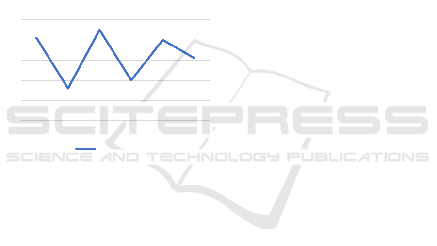
3.2 The Performance of the Various

Epochs

In Fig. 3, it can observe the contrasting MSE values

across different epochs, despite keeping the number of

LSTM layers constant. The line chart illustrates that

there isn't a notably strong correlation between the

epoch value and the accuracy of CO2 emission

forecasts. This phenomenon exemplifies the concept

of model convergence, where the model reaches its

optimal state. Once the model has attained this optimal

state, further training becomes unnecessary as it runs

the risk of overfitting. Overfitting occurs when the

model becomes too specialized to the training data,

leading to reduced accuracy when presented with new,

unseen data. In this case, increasing the epoch value to

20 results in a higher MSE value and lower accuracy,

mirroring the findings depicted in Fig. 3. It is

important to strike a balance between training the

model to capture meaningful patterns in the data and

avoiding overfitting. Determining the ideal epoch

value requires careful consideration and

experimentation to ensure optimal model performance.

Beyond a certain point, increasing the epoch value

may not yield significant improvements in accuracy

4,7

4,75

4,8

4,85

4,9

remove 1

layer

original layers add 1 layer

MSE Value

DAML 2023 - International Conference on Data Analysis and Machine Learning

530

and can potentially lead to computational

inefficiencies. By understanding the relationship

between epoch values, MSE values, and accuracy,

researchers and practitioners can employ this

knowledge to fine-tune their models and make

informed decisions when training LSTM networks for

CO2 emission prediction.

Therefore, adding additional training times does

not necessarily increase the precision of forecasts of

CO2 emissions. In the range of 5 to 50 epochs, epoch

10 is the most accurate, and epoch 20 is the least

accurate, as shown in Fig. 3. The graph does not show

a link between these two variables that is either direct

or inverse. Consequently, in order to acquire the

experiment's finest results, it is necessary to compare

the occurrences of different epochs.

Figure 3: Comparison of MSE values with different epochs

(Picture credit: Original).

4 CONCLUSION

This study introduces machine learning and deep

learning technology to contribute to more accurate

CO2 emission projections. The LSTM model is

introduced as a baseline. Additionally, this paper

analyzes the impact of different layers and iterations

of LSTM. Extensive experiments were conducted to

evaluate the proposed method. By comparing the

MSE values for various combinations of LSTM layers

and epochs, lower values signify estimates of CO2

emissions that are more precise. Experimental results

show that within a specific range, increasing the

LSTM layer can make the CO2 emission prediction

more precise, and the reliability of the CO2 emission

prediction is different and unstable when the training

times or epochs are different. The epochs in this

experiment with the smallest MSE value, or the

maximum prediction accuracy, are 10 epochs, which

comprises 5 to 50 epochs. In the future, experiments

with different hyperparameters like batch size and

adjusting the sequence length for the LSTM will be

considered the research objectives for the next stage.

The research will focus on how different batch sizes

and sequence lengths will affect the precision of CO2

emission prediction and what their relationship is.

Consequently, it is simple to find better and more

reliable models for projecting CO2 emissions to assist

organizations like governments in responding, even if

they are required to.

REFERENCES

S. I. Seneviratne, M. G. Donat, A. J. Pitman, et al.

“Allowable CO2 emissions based on regional and

impact-related climate targets,” Nature, vol. 529,

2016, pp. 477-483.

M. Reichstein, M. Bahn, P. Ciais, et al. “Climate extremes

and the carbon cycle,” Nature, vol. 500, 2013, pp.

287-295.

Y. Hu, Y. Man. “Energy consumption and carbon emissions

forecasting for industrial processes: Status,

challenges and perspectives,” Renewable and

Sustainable Energy Reviews, vol. 182, 2023, p.

113405.

B. W. Ang. “The LMDI approach to decomposition

analysis: a practical guide,” Energy policy, vol. 33,

2005, pp. 867-871.

Q. Wang, Y. Wang, Y. Hang, et al. “An improved

production-theoretical approach to decomposing

carbon dioxide emissions.” Journal of environmental

management, vol. 252, 2019, p. 109577.

C. Zhang, B. Su, K. Zhou, et al. “Decomposition analysis

of China's CO2 emissions (2000–2016) and scenario

analysis of its carbon intensity targets in 2020 and

2030,” Science of the Total Environment, vol. 668,

2019, pp. 432-442.

D. Fang, X. Zhang, Q. Yu, et al. “A novel method for

carbon dioxide emission forecasting based on improved

Gaussian processes regression,” Journal of cleaner

production, vol. 173, 2018, pp. 143-150.

A. Tealab, “Time series forecasting using artificial neural

networks methodologies: A systematic review,” Future

Computing and Informatics Journal, vol. 3, 2018, pp.

334-340.

L. Peng, L. Wang, D. Xia, et al. “Effective energy

consumption forecasting using empirical wavelet

transform and long short-term memory,” Energy, vol.

238, 2022, p. 121756.

A. Rostamian, J. G. O’Hara. “Event prediction within

directional change framework using a CNN-LSTM

model,” Neural Computing and Applications, vol. 34,

2022, pp. 17193-17205.

Dataset https://www.kaggle.com/datasets/txtrouble/

carbon-emissions.

4,6

4,7

4,8

4,9

5,1

5 epoch 10

epoch

MSE Value

The Prediction of Carbon Dioxide Emissions and Parameter Analysis Based on the LSTM

531