Machine Learning Utilized in Prognosis of Hypertension

Zihan Zhou

Facility of Science & Engineering, University of Liverpool, Liverpool, U.K.

Keywords: Machine Learning, Multi-Layer Perceptron, Hypertension Prediction.

Abstract: People are getting increasingly conscious of their physical health issues since their quality of life advances.

Computers empower the medical industry, making medicine gradually become visualized. The adverse effects

of hypertension in the human body are already well established. As more people become aware of this, they

desire to be able to figure out whether or not they have hypertension without consulting a doctor. The

development of digital health has given this castle in the sky a foothold on the ground. According to

hypertension, there are 13 influencing factors in total: age, sex, cp, trestbps, chol, fbs, restecg, thalach, exang,

oldpeak, slope, ca, thal. The method adopted in this article is to use a neural network model with the help of

Python. By changing the factor's weight, the critical alpha factor obtains a higher weight and classifies it more

efficiently and accurately. This article chooses a simple neural network model, Multi Layer Perceptron (MLP),

then uses the validation set obtained from the data set to optimize hyperparameters and improves it multiple

times to obtain suitable hyperparameters to establish an optimal MLP model.

1 INTRODUCTION

Machine learning is widely used in the biomedical field

to classify research subjects due to its excellent ability

to handle an abundance of data and efficiently discover

the direct relationship between different pathogenic

factors and diseases. Helping to identify potential

disease possibilities can assist patients in

understanding disease messages at the onset of illness,

receiving timely and effective treatment, and reducing

the incidence of death (Atkinson and Atkinson 2023).

Many universities have also established disciplines

to cope with the growing data management and

analysis skills in the medical industry and even help

with preliminary disease screening. For example,

University College London and the University of

Manchester have launched health data science majors

to respond to related talent needs.

Among various machine learning algorithms,

neural networks have always attracted attention. Take

the hypertension problem studied in this article as an

example. Neural networks have been used to process

data related to clinical hypertension and help observe

changes in early subclinical diseases. Such changes

are too subtle to be discovered manually; hence,

efficient computer algorithms can assist in screening

out disease patients. For example, the convolutional

neural network (CNN) algorithm is used to both

process electrocardiogram signals and perform

classification predictions based on the relationship

between the electrocardiogram signals and the

prevalence of hypertension (Kiat Soh et al 2020).

Neural network algorithms have been developed

for some time, and many types of neural networks

have been produced in order to suit different

environments, such as Kohonen Networks (KN),

Deep Residual Network (DRN), and Liquid State

Machine (LSM). MLP, as one of the simple neural

network algorithms, is worth exploring further.

Therefore, this paper applies MLP as an algorithm tool

for hypertension classification prediction, judging

whether the patient has hypertensive diseases

according to the factors.

2 RELATED WORK

Current algorithms for predicting hypertension

classification are mainly divided into two parts. Part

of it is traditional machine learning, such as logistic

regression (LR), support vector machines (SVM) and

K nearest neighbours (KNN) (Jahangir et al 2022 &

Shi et al 2022). The other part is deep learning derived

from machine learning, such as various neural

networks (Kiat Soh et al 2020, Jahangir et al 2022, Shi

et al 2022 & LaFreniere et al 2016).

Zhou, Z.

Machine Learning Utilized in Prognosis of Hypertension.

DOI: 10.5220/0012801300003885

Paper published under CC license (CC BY-NC-ND 4.0)

In Proceedings of the 1st International Conference on Data Analysis and Machine Learning (DAML 2023), pages 279-284

ISBN: 978-989-758-705-4

279

The earliest data using neural networks to predict

hypertension can be traced back to the paper written

by Poli, R. et al., which uses Artificial Neural

Networks (ANN) to explore the prediction effect of

feedforward network models under the construction of

2-layer, 3-3-layer and 6-layer networks (Poli et al

1991). Memory data and diastolic and systolic blood

pressure time throughout the day are used as input

values, and antihypertensive drug doses are used as

output values. Models that explore different levels of

complexity simulate the reasoning of doctors using

different diagnostic modalities (Poli et al 1991).

As mentioned earlier, the data mostly comes from

the subjects' memory data and blood drug

concentrations, which are variables that can be

directly linked to the prediction of high blood pressure.

However, some patients do not know they have

hypertension in real life because they do not take drugs.

The above methods are not very useful to them, so

some scholars have explored how to predict high

blood pressure from other angles.

Nematollahi, M.A. and others have taken a

different approach by focusing on body composition

index to see if it can predict high blood pressure

(Nematollahi et al 2023). The study used more than

ten algorithms in machine learning to classify the data

individually and look for the features most relevant to

high blood pressure among all the features

(Nematollahi et al 2023).

Although many factors are used as inputs in

machine learning, this is unreasonable, and some

factors are not very helpful for predicting

classification, such as the patient's ID number, age and

gender. A few or even one crucial indicator is enough

for doctors to infer whether the patient is ill. Too many

input variables will lead to problems such as

overfitting when the algorithm is used after learning,

and it also wastes the role of doctors in clinical

diagnosis, resulting in a waste of resources (Filho et al

2021).

3 METHOD: NEURAL

NETWORK MODEL

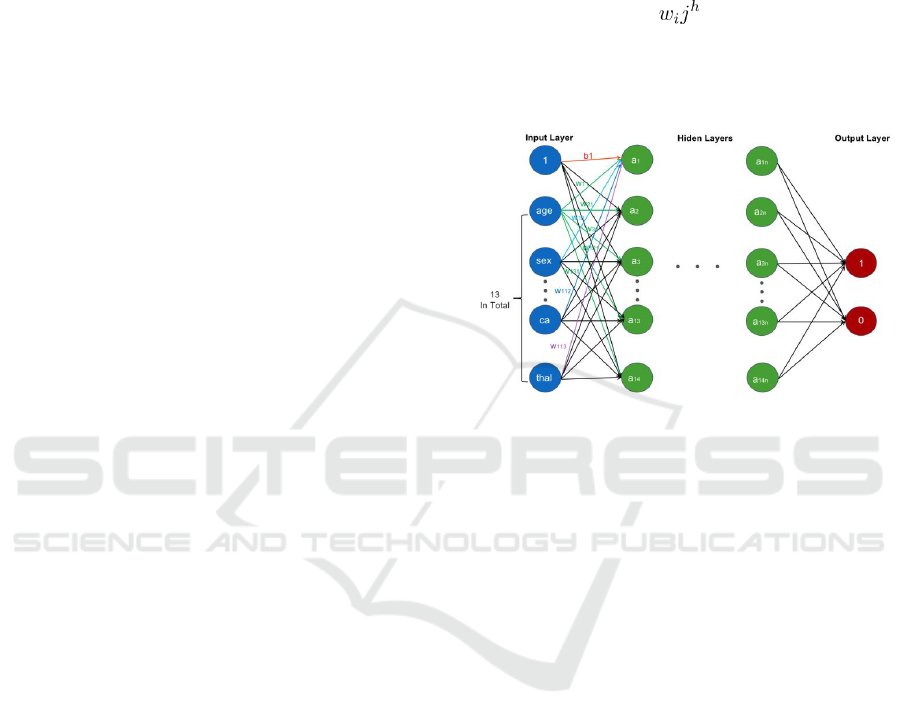
The input, hidden, and output layers are the three

primary components of the Multi-Layer Perceptron

neural network. As seen in Fig. 1, the input layer is the

first column, the output layer is the last, and the hidden

layer is everything in between (Rivas and Montoya

2020). According to the content of the dataset, the

input layer has a total of 13 input variables, that is, 13

factors related to hypertension. The number of hidden

layers is not specified here explicitly. Because

modifying the number of hidden layers is a variable in

the procedure of optimization and has an influence on

the model's accuracy. Finally, the output layer has

only two variables, 0 and 1. Having high blood

pressure is indicated by a score of 0, whereas

hypertension is indicated by a score of 1. Each column

is linked by weights, representing weights; i

represents the ith neuron in the next layer of the

network, j represents the jth neuron in the previous

network, and h represents the weight of the h layer

(Rivas and Montoya 2020).

Figure 1: MLP signal transmission between layers (Picture

credit: Original).

4 RESULT AND DISCUSSION

4.1 Data Set

4.1.1 Introduction to Data Sets

The dataset used in this article is from the Centers for

Disease Control (CDC) and Prevention using BRFSS

Survey Data from 2015 (Hypertension data set 2023).

In the extensive data framework of “Diabetes,

Hypertension and Stroke Prediction”,

hypertension_data.csv file was chosen as the dataset

for this study.

Use Python to read the imported hypertension data

and perform a numerical statistical description of the

stored framework to check whether the values are

missing and whether each feature is reasonably

distributed. From table I, the Sex item in the first row

is only 206058, which is 25 less than the other 206058

items, meaning there is a missing problem with the

data. After performing Python operations, it is found

that the missing items are all sex column data. The

data in the sex column are all 0-1 distributions

(Bernoulli distribution), with 0 representing females

and 1 representing males. The value returned is half of

DAML 2023 - International Conference on Data Analysis and Machine Learning

280

the total data for the sex item, which represents a

balanced gender balance. After running the

summation code, find that the number of men and

women is equal, both of which are 13029. The value

returned is half of the total data for the sex item, which

represents a balanced gender balance.

In this case, in order to avoid the impact of the

imbalance of male and female proportions on the

overall data set due to the completion of the data, the

selected exclusion data was used to adjust the data set.

Considering that only sex has missing data, exclude

any rows of data containing missing values.

Finally, the new dataset is checked and finished

without missing values.

4.1.2 Dataset Partition

As shown in Figure 2, dataset here has been divided

into 3 part: training set, validation set, and test set

according to the ratio of 7:2:1 utilized train_test_split

function.

Figure 2: TRAIN_TEST_SPLIT (Picture credit: Original).

The training set is used to fit the data to train the

model, the validation set is used to optimize

hyperparameters, and it can effectively avoid the

problem of overfitting or underfitting the training

model. Ultimately, the test set is invisible data to

simulate real-world information. The use of these

three sets reflects the model's behaviour, improving its

efficiency and accuracy and making it more relevant

to real-life applications.

After dividing the datasets, use the format function

to check the size and sample size of the three classified

sets.

4.2 MLPClassifier

For the data with good scores to enter the model for

subsequent optimization after learning, it is necessary

to separate the predictors (age to tha column) from the

three sets' answers (target column). X represents the

set of predictors, and Y represents the answer. After

training the model MLP using the train set, use the

trained model to predict the validation set and the

accuracy of the test set.

The result is that no matter how many times the

three collections are run, the classification accuracy is

always greater than 95%. Even more surprising is that

the difference in classification accuracy of the three

sets per run is minimal, no more than 0.5%. Even

sometimes the same rate of accuracy. This result

means the model will most likely have data leakage or

overfitting.

Table 1: MLP input factors.

age

sex

trestbps

chol

count

26083.00

26058.00

26083.00

mean

55.66

0.50

0.96

131.59

246.25

std

15.19

0.50

1.02

17.59

51.64

min

11.00

0.00

94.00

126.00

25%

44.00

0.00

120.00

211.00

50%

56.00

0.50

1.00

130.00

240.00

75%

67.00

1.00

2.00

140.00

275.00

max

98.00

1.00

3.00

200.00

564.00

fbs

restecg

thalach

exang

oldpeak

count

26083.00

mean

0.15

0.53

149.66

0.33

1.04

std

0.36

0.53

22.86

0.47

1.17

min

0.00

71.00

0.00

25%

0.00

133.00

0.00

50%

0.00

1.00

153.00

0.00

0.80

75%

0.00

1.00

166.00

1.00

1.60

max

1.00

2.00

202.00

1.00

6.20

slope

thal

target

count

26083.00

mean

1.40

0.72

2.31

0.55

std

0.62

1.01

0.60

0.50

min

0.00

25%

1.00

0.00

2.00

0.00

50%

1.00

0.00

2.00

1.00

75%

2.00

1.00

3.00

1.00

max

2.00

4.00

3.00

1.00

Machine Learning Utilized in Prognosis of Hypertension

281

4.3 Optimize Hyperparameters

The validation set precisely adjusts the parameters and

finds the best hyperparameter value.

When tuning, the optimized parameter is the

unique variable.

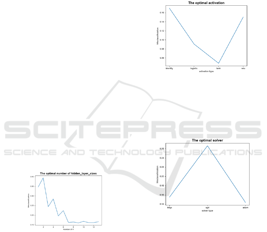
4.3.1 Hidden Layer Size Optimization

The dataset dictates the number of nodes in both the

input layer and output layer, which are the three

essential layers that make up a neural network. The

proper amount of layers and the quantity of hidden

layer nodes should be selected to optimize the neural

network's performance for either a regression or

classification job.

The impact is better the more layers there are, but

the more layers there are, the more overfitting issues

there may be, and the harder it is to train, which makes

it tougher for the model to converge.

It is essential to select the appropriate hidden layer

structure and the number of neurons, and this paper

uses grid search or cross-validation to determine the

optimal structure.

The line chart in Fig. 3 shows that the x-axis

represents the different H values (H represents the

number of hidden layers), and the y-axis represents the

misclassification rate. The increase in the number of

hidden layers dramatically improves the classification

accuracy, and after increasing to 7 layers, it tends to

stabilise and oscillate sideways within a specific range.

Based on this chart, it can be found that H=9 is the

best value for H.

Figure 3: The optimal number of hidden layer size (Picture

credit: Original).

However, a fixed number of layers seems like a

bad idea, and if the code runs multiple times, the

optimal hidden_layer_sizes will change the size.

Therefore, it is best to stabilise the hidden layer sizes

within a specific range. Depending on the size of the

input and output variables, the number of hidden

layers is specified between 2 and 14.

4.3.2 Activation Optimization

Consider Fig. 4 below, where the x-axis represents the

different activation types and the y-axis represents the

misclassification rate.

The line chart shows that the tanh function gives

the best performance.

Figure 4: The optimal activation (Picture credit: Original).

After running the algorithm many times, activation

is feasible. If the validation set is replaced with the

training or test set, the optimal activation will not

change; it has always been tanh.

4.3.3 Solver Optimization

Figure 5: The optimal solver (Picture credit: Original).

Sadly, a fixed number of layers does not seem like

a good idea, and if the size of the validation set

changed, the best solver would change, ibfgs will be

the best choice when the set is small, and adam for the

rest of the time based on Fig. 5.

4.3.4 Learning Rate Optimization

According to the Fig. 6, which illustrates the

misclassification rate under different learning rates,

the constant performs best according to the line.

DAML 2023 - International Conference on Data Analysis and Machine Learning

282

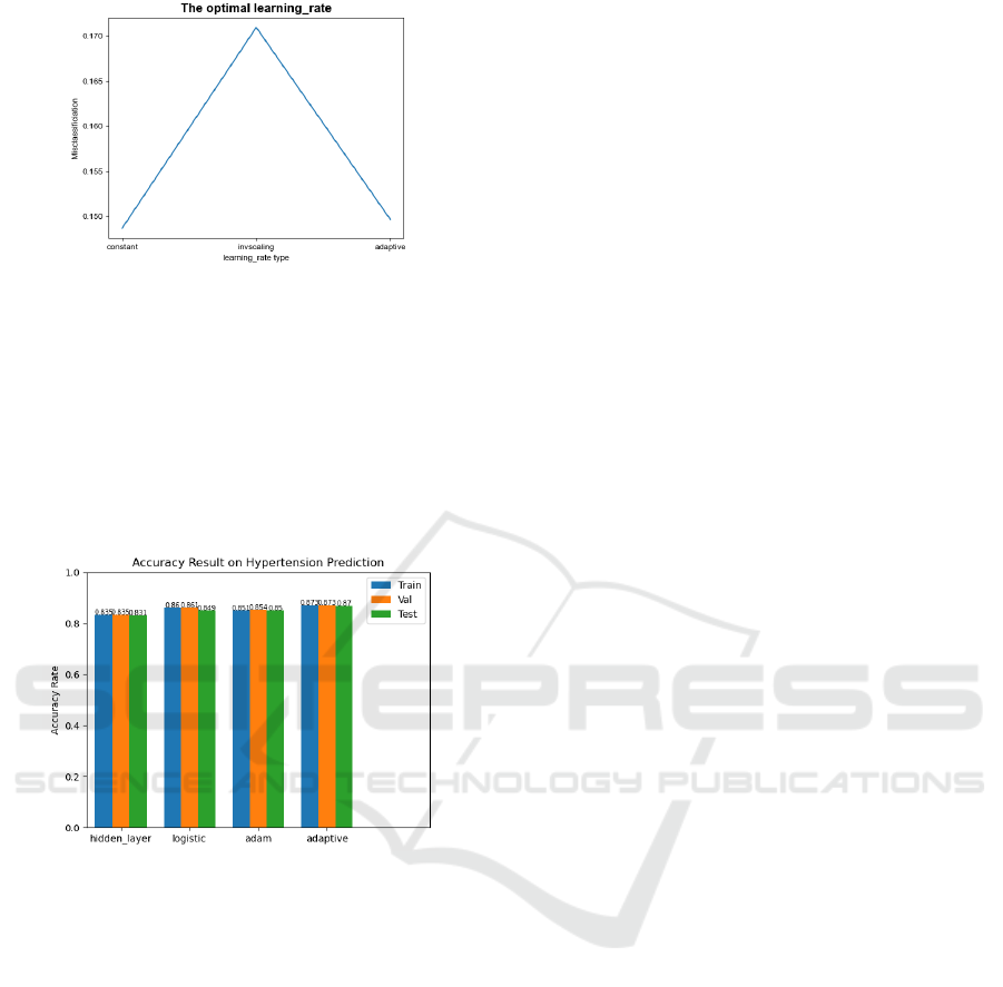
Figure 6: The optimal learning rate (Picture credit: Original).

4.4 Accuracy

Fig. 7 illustrates the accuracy of the model in

predicting hypertension classification. The x-axis

represents different hyperparameters, and the y-axis is

the accuracy. The parameters of the x-axis are run step

by step, which can control the accuracy of the overall

model.

Figure 7: Accuracy result on hypertension prediction

(Picture credit: Original).

The first set of histograms represented by

hidden_layer_sizes is different from running the MLP

model directly, and the accuracy rate is more than 95%,

but the accuracy rate here is less than 85%. This is

because when running the MLP model directly, the

default hidden layer sizes are up to 200, which will

cause the model layer to be too deep and overfitting,

and choosing a small number of hidden layers can

alleviate this problem.

The second set of histograms represents an

optimized activation function based on hidden layer

sizes, and unlike the optimized tanh function, the

logistic function is selected as the activation function.

Although the optimal activation function in the

optimization is the tanh function when combined with

hidden layer sizes, the accuracy of the overall model

will drop below 55%, so the choice of activation

function is problematic. So, after filtering, the

activation function is changed to logistic function,

which is also in line with the characteristics of logistic

function more suitable for classification algorithms.

The accuracy of the first and second histograms

increased but decreased slightly in the third group.

However, unfortunately, all solvers except Adam had

less than 55% accuracy in the overall model.

The last group represents the accuracy rate of the

model after the new learning rate and selects constant

as the learning rate when optimizing. Adaptive is

selected as the learning rate after many tests to match

the overall model. As a result, the accuracy of the

overall model increased step by step to 87%.

Although the optimal activation function here is

tanh, the accuracy rate when running the optimal

model is only 54.8%, which means that the choice of

activation function is incorrect, and the accuracy rate

after replacing the activation function with logistic has

increased significantly, about 87.3%.

5 CONCLUSION

This paper studies the effect of neural network

algorithm in hypertension prediction. First and

foremost, utilising the training set to fit the MLP

model. Then, the validation set is used for

hyperparameter optimisation. Finally, the appropriate

parameters are selected to generate the optimal MLP

model to improve the accuracy of the model. The

optimal model obtained by optimising the

hyperparameters can achieve 87% accuracy on the test

set. This accuracy rate shows that the model performs

well and that the blood pressure prediction results are

satisfactory.

Considering that different models need to be

suitable for different datasets (that is, there are

different classification factors), the model can be

applied to most cases, and the feedforward model can

learn the training set, generate appropriate weights,

weights help increase the importance of features that

are highly correlated with classification results, and

help classify data more reasonably.

The experiments in this article are not mature

enough and only consider all factors as variable inputs

and do not consider the need for reasonable clinical

use. Subsequently, five suitable and effective factors

can be screened out in advance to assist doctors in

screening. For example, hypertensive antihypertensive

drugs can be used as an essential factor and effectively

learned in combination with medical knowledge.

In addition, the optimisation of hyperparameters in

this paper still needs to be improved. MLP has many

parameters, but this paper only optimises a few of

Machine Learning Utilized in Prognosis of Hypertension

283

them, and more parameters can be optimised in the

future to produce better models.

REFERENCES

J. Atkinson and E. Atkinson, “Machine Learning and Health

Care: Potential Benefits and Issues,” Journal of

Ambulatory Care Management, vol. 46, no. 2, pp.

114-120, 2023.

Desmond Chuang Kiat Soh, E.Y.K. Ng, V. Jahmunah, Shu

Lih Oh, Ru San Tan and U. Rajendra Acharya,

“Automated diagnostic tool for hypertension using

convolutional neural network,” Computers in Biology

and Medicine, vol. 126 , 2020.

A. Jahangir, K. Tirdad, A. Dela Cruz, A. Sadeghian and M.

Cusimano, “An Application of Machine Learning to

Forecast Hypertension Signals in Intracranial

Pressure: A Comparison of Various Algorithms,”

IEEE systems, man, and cybernetics magazine, vol. 8,

no. 1, pp. 29-38, 2022.

Y. Shi, L. Ma, X. Chen et al., “Prediction model of

obstructive sleep apnea-related hypertension:

Machine learning-based development and

interpretation study,” Frontiers in cardiovascular

medicine, vol. 9, pp. 1-12, 2022.

D. LaFreniere, F.Zulkernine, D. Barber and K. Martin,

“Using machine learning to predict hypertension from

a clinical dataset,” 2016 IEEE Symposium Series on

Computational Intelligence, SSCI , 2016.

R. Poli, S. Cagnoni, G. Coppini and G. Valli, “A neural

network expert system for diagnosing and treating

hypertension,” Computer (Long Beach, Calif.), vol.

24, no. 3, pp. 64–71, 1991.

M. Nematollahi, S. Jahangiri, A. Asadollahi et al., “Body

composition predicts hypertension using machine

learning methods: a cohort study,” Scientific reports,

vol. 13, no. 1, pp. 6885-6885, 2023.

Chiavegatto Filho, A., Batista, A.F.D.M. and Dos Santos,

H.G. “Data Leakage in Health Outcomes Prediction

With Machine Learning. Comment on ‘Prediction of

Incident Hypertension Within the Next Year:

Prospective Study Using Statewide Electronic Health

Records and Machine Learning’ ,” Journal of medical

Internet research, vol. 23, no. 2, pp.1-4, 2021.

P. Rivas and L. Montoya, “Deep Learning for beginners a

beginner’s guide to getting up and running with deep

learning from scratch using Python,” S.l: Packt

Publishing, 2020.

Hypertension data set available at:

https://www.cdc.gov/brfss/annual_data/annual_2015

.html retrieved on September 1, 2023.

DAML 2023 - International Conference on Data Analysis and Machine Learning

284