The Investigation of Packet Header Field Importance on Malware

Classification following Nprint Processing

Fangzhou Xing

Department of Math Major, Swarthmore College, Swarthmore, U.S.A.

Keywords: Malware Classification, Nprint, Machine Learning.

Abstract: In 2021, a research endeavor aimed to standardize and automate the utilization of machine learning in network

traffic analysis through the introduction of Nprint. Nprint converts complete packets into binary representation

(1s, 0s, and -1s), subsequently feeding the processed data into an autoML system. This study demonstrated

remarkable performance across various network traffic analysis tasks, including malware classification.

However, it did not investigate the impact of excluding certain packet header fields on the results.

Consequently, this research seeks to explore how the utilization of Nprint for data processing, while

selectively considering specific packet header fields, influences the outcome of the malware classification

task. This research used random forest on Nprint processed network traffics to determine the importances of

each header field on the task of malware classification, and then tried using only the information of top n most

important header fields as the data to be fed into AutoGluon to determine how the classification accuracy and

the training time would be changed. The research had found that using only 3 of the packet header fields could

still achieve an accuracy that was 99.9% of the accuracy achieved by using all the header fields, and at the

same time shortened the training time required for the best performing modal on this task given by an

AutoGluon by more than half.

1 INTRODUCTION

Since the advent of the Digital Age, computer users

have faced an ongoing threat from malware, which are

malicious software programs designed to inflict harm

on computer systems, seek unlawful financial gain,

compromise personal privacy, and more. From the

early malwares like the Creeper Worm to the modern

malwares like NotPetya, malware threats have been

growing both in magnitude and diversity alongside the

development of technology (Gibert and Mateu 2020).

In the current society in which the internet and smart

devices play increasingly vital roles, there is a growing

demand for cyber security and malware detection.

According to statistics, there are 23.14 billion Internet

of Things devices connected across the world in 2018,

and this number is projected to grow rapidly (Hussain

2021). While at the same time, a report has shown that

there are about 5.4 billion malware cyber attacks in

2021 (SonicWall 2022).

In an effort to protect individuals and institutions

from the harm of malware, researchers have been

researching on methods to detect and classify malware.

One of the directions is analysing network traffic flows

and detecting malicious traffics (Gibert and Mateu

2020). For the last decades, in the backdrop of the

flourishment of machine learning, there has been an

increasing number of researches on employing

machine learning techniques to detect and classify

malware (Gibert and Mateu 2020). Machine learning

has demonstrated its effectiveness in various domains,

exemplified by the triumph of AlphaGo, a Go-playing

program that defeated world champions (Silver et al

2017). Not surprisingly, machine learning techniques

have also shown to be useful in malware traffic

detection and classification. For example, research

employed a Long Short-Term Memory (LSTM)

classifier which takes HyperText Transfer Protocol

Secure (HTTPS) traffic as input to determine whether

the flow is from a malware (Machlica et al 2017).

There are abundant of benchmarks and challenges

provided for studies of the applications of machine

learning in other more popular fields like Computer

Vision or Natural Language Processing, but

benchmarks and challenges for study of network traffic

are lacking (Barut et al 2020). In response to this

problem, the research collected a dataset of about 500

thousand network flow samples, which were

Xing, F.

The Investigation of Packet Header Field Importance on Malware Classiﬁcation Following Nprint Processing.

DOI: 10.5220/0012808500003885

Paper published under CC license (CC BY-NC-ND 4.0)

In Proceedings of the 1st International Conference on Data Analysis and Machine Learning (DAML 2023), pages 343-348

ISBN: 978-989-758-705-4

343

categorised into 19 malware classes and 1 benign class,

for researchers to use and to compare their results on

Holland’s study in 2021. The study also engineered

these network flows into flow features for the research

community to work with Barut’s study in 2020.

A study in 2021 seeks to further simplify the data

preparation and feature engineering part of the

machine learning pipeline in network traffic analysis,

including malware traffic analysis, through the

introduction of NprintML (Holland et al 2021).

NprintML is divided into two parts, Nprint and

AutoML (Holland et al 2021). Nprint transforms raw

packets into a standard binary representation with -1

paddings to keep packet header fields aligned

(Holland et al 2021). AutoML are libraries which

select and tune differently machine learning modals

automatically based on the input (Holland et al 2021).

With NprintML, the study seeks to standardise and

automate the machine learning process, without the

need for expert knowledge on what feature or packet

header field is important (Barut et al 2020). The study

showed superior results on many network traffic

analysis tasks. However, the study did not provide

insights into the potential outcomes when specific

packet header fields are chosen for processing by

Nprint in various tasks, such as malware analysis.

Therefore, this research will study how choosing

only certain packet header fields to be processed by

Nprint and later by autoML will affect the accuracy

of malware classification. The study will first use

random forest algorithm to analyse the importance of

each work. Then the study will choose different sets

of packet header fields to be processed by Nprint and

autoML and compare their results with using all

packet header fields.

2 METHOD

2.1 Dataset Preparation

The dataset used in this research is a subset of the

dataset used by the malware detection section of the

Nprint study (Holland et al 2021). The original data

contains approximately 500, 000 traffics of packets,

each being labelled by the classification it is in

Holland’s study in 2021. The largest traffics contain

100 packets and the smallest traffics contain only 1

packet (Holland et al 2021). Out of the approximately

500, 000 traffics in the dataset, there are just over 170,

000 traffics that contain at least 10 packets (Holland

et al 2021). This research uses 170, 000 traffics that

contain at least 10 packets from the original dataset.

The 170, 000 traffics first had their packets being

turned into rows of 1s 0s and -1s through Nprint

(Holland et al 2021). Each row of 1s 0s and -1s

represents one packet and each column of of 1s 0s and

-1s represents one sub-feature (Holland et al 2021).

Each packet had 960 sub-features, and the sub-

features group together to represent 36 features,

which are the 36 header fields of the protocols ipv4,

tcp, udp for each packet (Holland et al 2021). The

header fields are shown in Table 1.

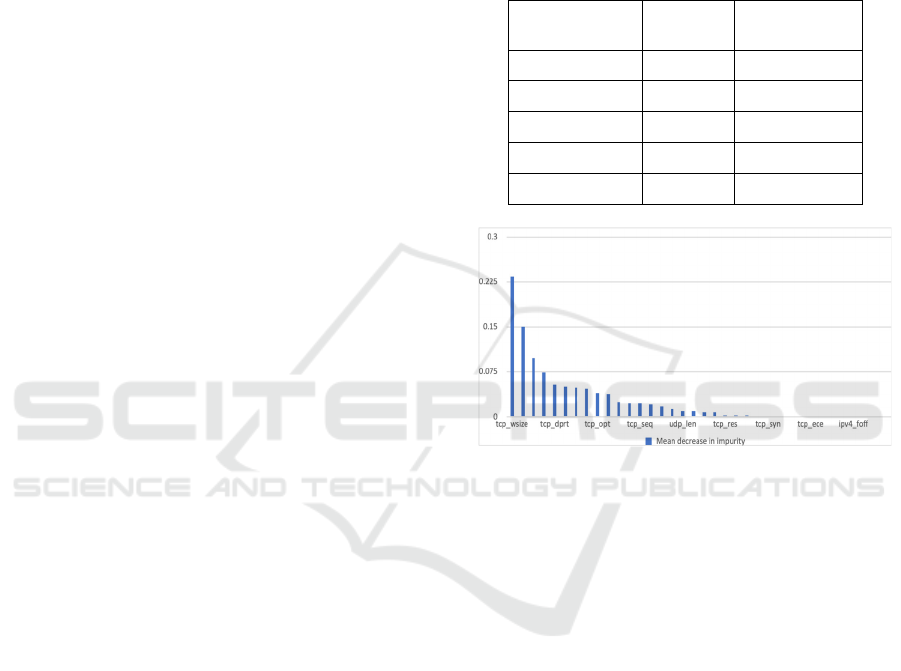
Table 1: Feature importance for each header field.

Header field Mean decrease in Impurity

tcp_wsize 0.233956

ipv4_tl 0.151328

ipv4_cksum 0.098145

ipv4_ttl 0.074087

tcp_dprt 0.054195

tcp_sprt 0.050146

tcp_psh 0.048142

ipv4_dfbit 0.046672

tcp_opt 0.039076

tcp_fin 0.037534

ipv4_id 0.024555

tcp_ackn 0.022336

tcp_seq 0.022046

tcp_cksum 0.021803

tcp_doff 0.018283

udp_cksum 0.013158

udp_len 0.009789

udp_dport 0.008867

tcp_rst 0.007856

udp_sport 0.006926

tcp_res 0.002776

ipv4_tos 0.002774

tcp_ackf 0.001793

tcp_ns 0.001049

tcp_syn 0.000931

tcp_cwr 0.000816

tcp_urg 0.000502

tcp_urp 0.000442

tcp_ece 0.000013

ipv4_hl 0.000000

ipv4_opt 0.000000

ipv4_proto 0.000000

ipv4_foff 0.000000

ipv4_mfbit 0.000000

ipv4_rbit 0.000000

ipv4_ver 0.000000

DAML 2023 - International Conference on Data Analysis and Machine Learning

344

The packets of each traffic were sorted by the time

they were received or sent. Then, since some study

showed that only inspecting the first few packets of

each traffic flow is sufficient for the purpose of

malware detection, and to keep the input size of each

traffic sample for machine learning consistent, only

the first 10 packets of each traffic was kept (Hwang

et al 2019). Next, for each traffic, its 10 packets were

placed side by side so that each row of 9600 sub-

features represents one sample. This is the standard

representation for each sample in this research. In the

experiments, the samples will be changed by

including and excluding groups of sub-features based

on the set of features chosen to be tested on.

The 170, 000 samples of processed labeled traffic

were split into 120, 000 training samples and 50000

testing samples. There are 19 categories for the 170,

000 sample. However, some categories didn’t have

many samples in them. Therefore, only the 10

categories that contained the most samples was

considered. The 10 categories are benign,

magichound, htbot, trickster, ursnif, artemis, trickbot,

dridex, emotet, minertorjan. After only considering

these 10 categories, there were 117842 samples for

training and 49124 samples for testing.

Before using the samples for training and testing,

the importance of each of the 36 features in malware

classification was determined through random forest

using sklearn (Pedregosa et al 2018). The set of

samples used to determine feature importance was all

of the samples in the training set. The 117842 samples

were adjusted to be suited for random forest. The

9600 sub-features were grouped to form 360 features,

which are the 36 header fields for each of the 10

packets in each sample. Then, the binary values for

features ipv4_hl, ipv4_tl, ipv4_foff, ipv4_ttl,

ipv4_cksum, tcp_seq, tcp_ackn, tcp_doff, tcp_wsize,

tcp_cksum, tcp_urp, udp_len, udp_cksum were

turned into base 10 integers, since these features

represent certain kinds of magnitude. The rest of the

features had their binary values turn into strings.

Then, since sklearn random forest only takes in

numerical inputs, the features with string values were

expanded to multiple features using one-hot

encoding. After the expansion, the samples had 1, 933

features.

2.2 Random Forest

2.2.1 Decision Tree

Decision tree is a binary tree for classification tasks

that contains two types of nodes: decision node and

leaf node. The tree starts from a decision node, which

represents a feature that contains a split of its

variables that gives the most information (Computed

using the training samples) gained compared to other

features. Then, the decision node is connected to two

child nodes by two edges each representing one set of

the variables formed by the split. The two-child node

can either be a leaf node, which represents one of the

categories in the classification, if all samples

satisfying all the conditions set by the ancestors of

this node are in this category, or another decision

node chosen by the same way its ancestors were

decided given the conditions set by its ancestors. The

tree is expanded with the above process until it cannot

be expanded.

This research used gini index to measure the

information gain caused by a split of variables for any

particular feature. Gini index of a node is calculated

by the function:

𝐺𝑖𝑛𝑖𝐼𝑛𝑑𝑒𝑥 =1−∑𝑝





(1)

In which

𝑝

𝑖

represents the probability for the

samples to be in category

𝑖 given that the samples

satisfy all the conditions set by the ancestors of the

node.

Information Gain is calculated by the function:

𝐼𝐺 = 𝑤



𝐺(𝑝𝑎𝑟𝑒𝑛𝑡) −∑𝑤



𝐺(𝑐ℎ𝑖𝑙𝑑



) (2)

In which

𝐺 is the gini index, 𝑤

𝑝

is the proportion

of samples satisfying all the conditions set by the

ancestors of the parent, and

𝑤

𝑖

is the proportion of

samples satisfying all the conditions set by the

ancestors of child

𝑖.

2.2.2 Random Forest

Random forest is a collection of n trees each trained

using a set of samples that had the same size as the

entire training set and had its samples chosen

randomly from the training set with replacement. The

features considered by each tree were selected

without replacement from all the features. The

number of features considered by each tree was the

square root of the total number of features. After

training the n trees, classification task was done by

giving the input to all n trees and then chose the

category that most trees gave as the result. In this

research, 100 trees were trained in the random forest.

2.2.3 Feature Importance

The feature importance of each feature in each tree

was calculated by taking the sum of the information

gain caused by all instances of decision nodes that

The Investigation of Packet Header Field Importance on Malware Classiﬁcation Following Nprint Processing

345

corresponds to that feature and then divided by the

sum of information gain caused by all nodes. The

normalised value of feature importance of each

feature in each tree was calculated by dividing the

feature importance of the feature by the sum of the

feature importance of all features. The feature

importance of each feature in the random forest was

the meaning of the normalised feature importance of

the feature in each tree. This value is also called the

mean decrease in impurity of the feature. This

research wanted to find out the importance of the

header fields, which were expanded to 1933 features

for the random forest. Therefore, the importance, or

the mean decrease in impurity, of each header field

was calculated by summing up the feature importance

of all the features related to that header field.

2.3 AutoML

AutoML were libraries that seeks to automate the

process of applying machine learning to solve

problems. Machine learning had been shown to be

useful in many areas and an increasing number of

research field or real life applications made use of it.

However, traditionally the application of machine

learning required expert knowledge, including

knowledge about data processing, model selection,

model hyperparameters tuning etc., to successfully

achieve the goals. These knowledge tends to take time

and practice to acquire. AutoMLs, by automating the

process of machine learning application, aimed to

simplify the usage of machine learning for non-

machine learning experts. AutoMLs allowed

researchers to be able to focus more on their own

research interests rather than spending time working

on model design or hyperparameter tuning that might

not be related to the aim of their research. This

research used Autogluon which was an autoML that

trains and tests multiple models and automates the

hyperparameter tuning process in model training

(Erickson et al 2020).

RESULTS

The importance of each header field calculated

through sklearn random forest feature importance

was showed in Figure 1 and Table 1. The 5 most

important header fields are tcp_wsize, ipv4_tl,

ipv4_cksum, ipv4_ttl, and tcp_dprt, with the most

important header field tcp_wsize having 0.233956

mean decrease in impurity.

This research first used AutoGluon to train 12

different models with all header field included. The

performance of the top 5 best performing models was

shown in Table 2. The best performing model was

NeuralNetFastAI, which had an accuracy of 0.978666

with a fitting time of 334.879 seconds. Out of the 5

best performing models, LightGBM had the shortest

fitting time, which is 48.920 seconds.

Table 2: Top 5 model performance (All header fields

included).

Model Accuracy

Fitting time

(seconds)

NeuralNetFastAI 0.978666 334.879

LightGBMXT 0.976264 79.691

LightGBM 0.975470 48.92

XGBoos

0.975307 133.913

CatBoos

0.975124 774.513

Figure 1: Header field importance using MDI

(Photo/Picture credit: Original).

Since, the model NeuralNetFastAI gave the best

accuracy out of the 12 models, this research decided

to train NeuralNetFastAI to show how samples that

included different header fields affect accuracy and

fitting time. The results were shown in Figure 2. The

figure showed three plots, accuracy, normalised

accuracy, and normalised fitting time with respect to

including top n most important header fields.

Accuracy was defined as the total number of correct

classifications over the total number of classifications

made. Normalised accuracy was the accuracy of the

sample over the accuracy of the sample that included

all header fields. Normalised fitting time was the

fitting time of the sample over the fitting time of the

sample that included all header fields. Figure 2 and

Table 3 showed that the accuracies of

NeuralNetFastAI using samples that included 3 or

more most important header fields had no significant

difference. While at the same time, there were

significant decrease in fitting time for samples that

included 15 or less most important header fields. With

only using the top 3 header fields, the accuracy was

DAML 2023 - International Conference on Data Analysis and Machine Learning

346

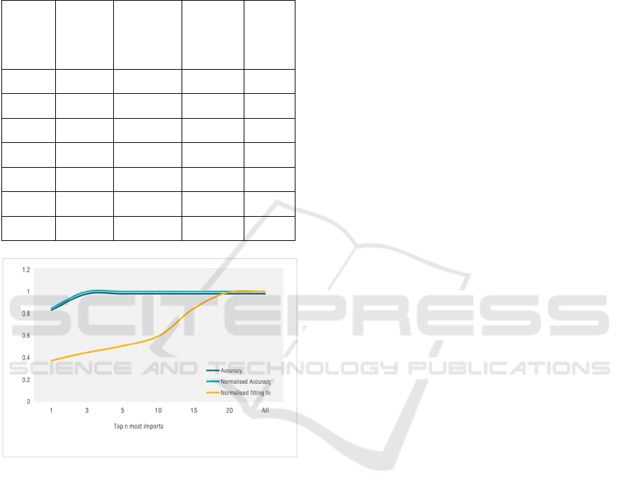
0.977465, 99.9 percent of the accuracy of using all

header fields, but the fitting time was only 149.110

seconds, 44.5 percent of the fitting time used when

including all header fields.

Table 3: Accuracy and fitting time for different # of header

fields included.

# of

header

field

include

Accuracy

Normalised

Accuracy

Normalised

fitting time

Fitting

time

1 0.830248 0.848347 0.371663 124.462

3 0.977465 0.998773 0.445265 149.110

5 0.978239 0.999564 0.504675 169.005

10 0.978503 0.999833 0.593277 198.676

15 0.977933 0.999251 0.844884 282.934

20 0.978707 1.000042 0.994389 333.000

ALL 0.978666 1.0 1.0 334.879

Figure 2: Comparison between normalised accuracy and

normalised fitting time using nodal NeuralNetFastAI

(Photo/Picture credit: Original).

Therefore, this research found that the task of

malware detection, with the given samples processed

using Nprint, only needs information about 3 header

fields to achieve accuracy comparable to the accuracy

achieved by using all 36 header fields. And by only

using 3 header fields, the fitting time for

NeuralNetFastAI is reduced by more than half.

4 DISCUSSION

The results showed that tcp_wsize, ipv4_tl,

ipv4_cksum, ipv4_ttl, tcp_dprt, and tcp_sprt are the

six most important header fields to be considered in

the malware classification task on the sample this

research used. tcp_dprt was the fifth most important

and tcp_sprt was the sixth most important. tcp_dprt

and tcp_sprt have similar importance confirmed with

intuition since the sample traffics contain packets

going in both directions, which meant that a port was

both used as a destination port and as a source port in

a traffic. Port number’s importance in malware

detection and classification might be due to the fact

that there were certain ports that were easy to be used

by certain attacks based on the ports’ specific security

weaknesses. Some attackers might make the total

length value in the header field vary short and

mismatch the actual length of the packet to trick

firewalls, which could be a possible reason for the

importance of ipv4_tl in malware classification. A

possible reason for ipv4_ttl to be one of the important

header fields was that ipv4_ttl could show

information about the number of hops the packet went

through before reaching destination, which might

give information on where the packet was from.

ipv4_cksum was a value that could help verify

whether the content of the packet had no error and had

not been changed. So if ipv4_cksum value showed

problems, then the packet could possibly be from a

traffic that was not normal. tcp_wsize didn’t seem to

have an intuitive reason why it was related to malware

traffic, but future studies might look more into it by

looking at the distributions of tcp_wsize for each

malware category. By looking at the machine

learning results for including selected header fields, it

seemed that it was not necessary to include all header

fields for the task of malware classification, but only

including the few most important ones would achieve

similar accuracy and at the same time saving a

considerable amount of modal training time.

5 CONCLUSION

In this study, the importance of individual header

fields in the context of malware classification was

assessed using a random forest model. Subsequently,

AutoGluon was employed to investigate how the

selection of different sets of header fields impacts

both accuracy and training duration. The research

identified the top five header fields critical for

malware detection as tcp_wsize, ipv4_tl,

ipv4_cksum, ipv4_ttl, and tcp_dprt. Interestingly,

utilizing only these selected header fields in samples

yielded comparable accuracy in malware

classification compared to using the entire set of

header fields, while significantly reducing training

The Investigation of Packet Header Field Importance on Malware Classiﬁcation Following Nprint Processing

347

time by over 50%. However, the importance of each

header field calculated in this research may not gave

a precise or exhaustive reflection of how important

each header field was, and more information about

each header field can be analysed. For example, some

header field might be very useful for the detection of

a particular malware category but not others. This

possibility was not reflected in the importance scores.

Also, in the circumstances in which a header field is

important for only the detection of a particular

malware category, the number of samples in that

category would affected the calculated importance

value for that header field. Therefore, more

investigations could be done to analyse how header

fields were related to each malware category in the

future.

REFERENCES

D. Gibert, C. Mateu, J. Planes, Journal of Network and

Computer Applications, vol. 153, 2020.

F. Hussain, S. Abbas, G. Shah, I. Pires, U. Fayyaz, F.

Shahzad, N. Garcia, E. Zdravevski, Sensors, vol. 21,

pp. 3025, 2021.

D SonicWall Cyber Threat Report, SonicWall, Inc, 2022.

D. Silver, J. Schrittwieser, K. Simonyan, I. Antonoglou, A.

Huang, A. Guez, T. Hubert, L. Baker, M. Lai, A.

Bolton, Y. Chen, T. Lillicrap, F. Hui, L. Sifra, G.

Driessche, T. Graepel, D. Hassabis, Nature, vol. 550,

pp. 354, 2017.

L. Machlica, T. Pevny, J. Havelka, T. Scheffer, IEEE. SPW,

pp. 205, 2017.

O. Barut, Y. Luo, T. Zhang, W. Li, P. Li, arXiv. cs. CR,

2020.

J. Holland, P.Schmitt, N. Feamster, P. Mittal, CCS ‘21, pp.

3366, 2021

R. Hwang, M. Peng, V. Nguyen, Y. Chang, Applied

Sciences, vol. 9, pp. 3414, 2019.

F. Pedregosa, G. Varoquaux, A. Gramfort, V. Michel, B.

Thirion, O. Grisel, M. Blondel, A. Muller, J.

Nothman, G. Louppe, P. Prettenhofer, R. Weiss, V.

Dubourg, J. Vanderplas, A. Passos, D. Cournapeau,

M. Brucher, M. Perrot, E. Duchesnay, arXiv. cs. LG,

2018.

N. Erickson, J. Mueller, A. Shirkov, H. Zhang, P. Larroy,

M. Li, A. Smola, arXic. stat. ML, 2020

DAML 2023 - International Conference on Data Analysis and Machine Learning

348