Evaluating ARIMA and LSTM Approaches for Predicting S&P 500

Index Movements: A Comparative Analysis

Keming Zhang

The Institute of Data Science, University of Rochester, Rochester, N.Y., U.S.A.

Keywords: ARIMA, LSTM, S&P 500, Time Series.

Abstract: Within the sphere of equity market trading, precise price prediction is paramount for steering investment

strategies and increasing returns. This manuscript presents a comparative study of two renowned time series

forecasting models, the AutoRegressive Integrated Moving Average (ARIMA) model and the Long Short-

Term Memory (LSTM) model. Given the S&P 500's significance as an investor benchmark, this study

employs historical S&P 500 price data from 2018 to 2023 to appraise the predictive efficacy of both ARIMA

and LSTM models. The findings in this instance underscore the superior precision of the ARIMA model over

the LSTM model. Nevertheless, it is imperative to highlight that the selection between ARIMA and LSTM

models ought to be dependent on the specific attributes of the data and the forecasting horizons in question.

This investigation illuminates the respective advantages and limitations of both models, offering valuable

insights for investors and scholars traversing the multifaceted terrain of financial markets. Subsequent

research could extend this inquiry by investigating additional time-series models to improve the proficiency

of stock price prognostications.

1 INTRODUCTION

As a popular investment avenue, the stock market

consistently garners significant attention from

investors. Accurate stock price forecasting

substantially aids investors in making informed

decisions, thereby enhancing their investment returns

(Gaiwen and Shihan 2023). For instance, in the stock

market, stock indices represent hypothetical

portfolios of investment holdings, and provide broad

representations of various financial market segments.

Consequently, both individual and institutional

investors often show greater interest in these indices

than in the standalone stock price of a specific

company (Young et al 2023 & Wang et al 2012). One

of the well-known stock indexes is the Standard &

Poor’s 500 (S&P 500) index, which was launched in

1957, and features the top 500 U.S. publicly traded

companies primarily ranked by market capitalization

(Kenton 2021). Given these circumstances, the S&P

500 is a highly representative stock index in the

United States and will be used as the data source for

the paper. In addition, to get more profit and suffer

less loss, thousands and millions of investors would

like to use the historical price of the stock index to

predict its future prices, but what predicting method

should they use always becomes a greatly stumping

problem.

Time series models are techniques that primarily

leverage historical data to predict future data values

(Tableau 2023). The stock price series is essentially a

time series that has properties like trends, cycles,

timelines, and so on (Gaiwen and Shihan 2023).

Therefore employing time series forecasting could be

a viable solution. Considering the aforementioned

reasons, it is logical for this paper to utilize the S&P

500 price as the dataset and employ time series

forecasting models for predictions. Specifically,

Section 2 of this paper introduces two fundamental

time series models, the Autoregressive Integrated

Moving Average (ARIMA) model and the Long

Short-Term Memory (LSTM) model. The subsequent

sections utilize these models for prediction in Section

3, discuss the results of the two models in Section 4,

and finally draw conclusions in Section 5.

444

Zhang, K.

Evaluating ARIMA and LSTM Approaches for Predicting S&P 500 Index Movements: A Comparative Analysis.

DOI: 10.5220/0012808700003885

Paper published under CC license (CC BY-NC-ND 4.0)

In Proceedings of the 1st International Conference on Data Analysis and Machine Learning (DAML 2023), pages 444-450

ISBN: 978-989-758-705-4

2 DATA & METHODOLOGY

2.1 Data Collection

The dataset, as shown in Table 1 (Ameri 2023),

utilized in this study comprises daily data information

on the S&P 500 stock index. The dataset includes 6

columns: ‘Date’ indicating the dataset's index, ‘Open’

indicating the stock's opening price on the current day,

‘High’ indicating the stock's highest price on the

current day, ‘Low’ indicating the stock's lowest price

on the current day, ‘Close’ indicating the stock's

closing price on the current day, and ‘Volume’

indicating the volume of stock traded on that day. The

dataset comprises 1260 rows, with each row

individually presenting unique information about the

stock index for each trading day from March 7th,

2018 to March 5th, 2023 (Garlapati et al 2021).

2.2 Arima Model

The ARIMA model posits that the future value of a

variable is linearly related to its past observations and

past random errors. This model, as introduced by Box

and Jenkins in 1970, is one of the most commonly

used time series models in the financial market for the

short run. This linear relationship can be expressed as

in (1):

0 1 1 2 2 1 1 2 2

... ...

t t t p t p t t t q t q

Y Y Y Y

          

− − − − − −

= + + + + + − − − −

(1)

To understand this function, it is known that 



and





are the actual value and the random error of a

certain variable at time period t, respectively. Then,





 



     



are the past values of the variable,

and 



 



     



are the past errors of the

variable. Finally, 



        and 



   

      are their coefficients (Ariyo et al 2014).

In simpler terms, three primary parametric

components—auto-regression (AR), integration (I),

and moving average (MA)—could be generated based

on this linear function of the ARIMA model. AR

signifies the weighted moving average over the prior

observations, I signify the linear or polynomial trend,

and MA signifies the weighted moving average over

the prior errors. These three components can be

represented by the abbreviated form ARIMA(p,d,q).

Here, p stands for the number of the auto-regressive

terms, d for the quantity of differencing (integrating)

required to stabilize the time series, and q for the

quantity of the moving average term (Wang et al 2012

& Guha and Bandyopadhyay 2016). This encapsulates

the fundamental concept of the ARIMA model.

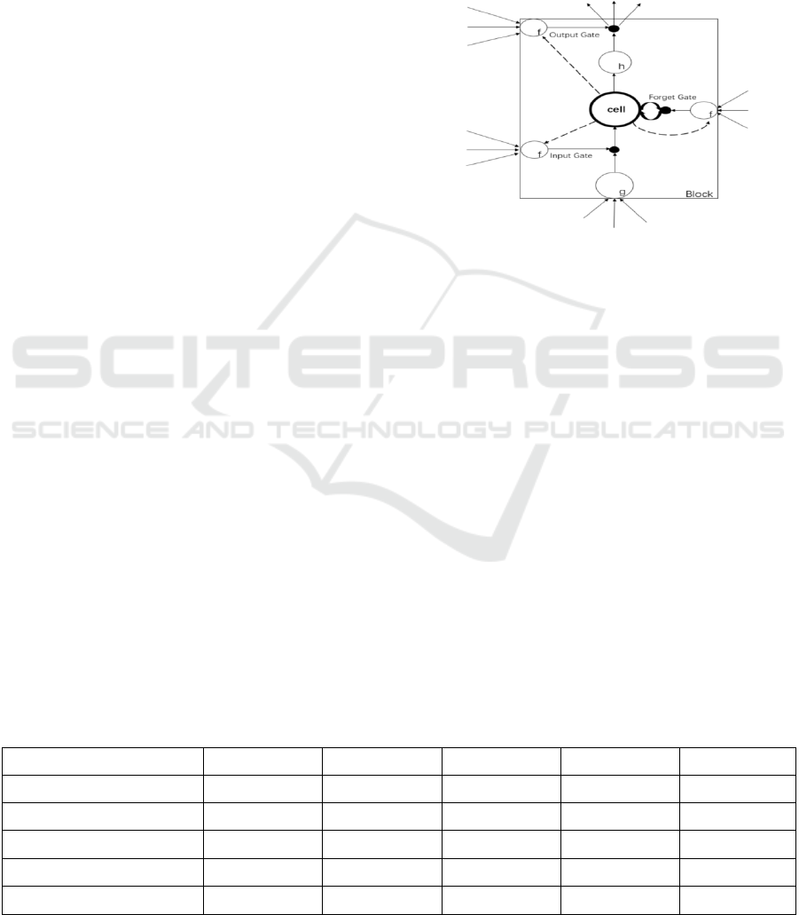
Figure 1: Structure diagram of LSTM.

2.3 Long Short-Term Memory (LSTM)

Model

The LSTM (Long Short-Term Memory) model was

proposed by Sepp Hochreiter and Jürgen

Schmidhuber in 1997. Originating from the

traditional Recurrent Neural Network (RNN) model,

the LSTM model was designed to address the issues

of vanishing or exploding gradients in the RNN

(Hanqing 2023). The LSTM model proves

particularly useful for time series prediction

involving long sequences of data and has been

utilized and refined by numerous researchers during

the past few years.

Then, it is necessary to see the concrete structure

of the LSTM model. According to Figure 1 (Haowei

2023), the LSTM model is mainly composed of 4 key

elements, which are memory cell, forget gate, input

gate, and output gate. The first thing to do in the

model is the forget gate operation, to decide which

Table 1: Original Dataset (Ameri 2023).

Date

Open

High

Low

Volume

2018-05-07

2680.340088

2883.350098

2664.699951

2672.629883

3266810000

2018-05-08

2670.260010

2676.340088

2655.199951

2671.919922

3746100000

2018-05-09

2678.120117

2676.340088

2674.139893

2697.790039

3913660000

2018-05-10

2705.020020

2726.110107

2704.540039

2723.070068

3380640000

2018-05-11

2722.699951

2732.860107

2717.449951

2727.719971

2874850000

Evaluating ARIMA and LSTM Approaches for Predicting S&P 500 Index Movements: A Comparative Analysis

445

parts of the content in the cell state need to be

discarded. The forget gate processes the current

input 



and the previous hidden state 



using the sigmoid function to generate a vector 



that ranges between 0 and 1. The vector 



calculated by (2). After discarding certain content, the

model proceeds to the second step: the input gate

operation. This operation determines what new

information from the current input should be retained

and transferred to the cell state. This operation includes

two steps. The first step is to use an S-shaped network

layer to examine the new information and get the

updated output of this gate 



,which is calculated by

(3). The second step involves using a tanh-activated

network layer to create a new candidate vector 



. This

vector is also used in the input gate operating process,

and is calculated by (4). Finally, the LSTM model

reaches its last step, which involves generating a

selective output of the current cell state through the

output gate. The final output 



can be calculated as

in (5) (Haowei 2023). Thus, this is the general concept

of the LSTM model.





  







 











()





  







 











()





  







 











()





  







 











()

3 PROCEDURE & RESULT

Having introduced the theoretical foundations of the

ARIMA and LSTM models, the paper will

subsequently utilize S&P 500 index data to concretely

illustrate the building steps of these two models and

their respective forecasting results.

3.1 Procedure and Results of the

ARIMA Model

This section of the paper employs the previously

mentioned data to detail the primary procedure for

building the ARIMA model and to present its

prediction results.

3.1.1 Data Preprocessing

Data preprocessing is about processing the original

data and generating a proper dataset which is in a

format suitable for time series analysis. The data must

undergo two main steps before being utilized in the

ARIMA model.

a) First Step - Choose Variables: It is necessary

to choose two variables used in this paper to do the

time series prediction, instead of using all 6 variables

shown in the original data. One of the variables should

represent the date to delineate the timeline, while the

other variable is preferably the closing price of the

S&P 500 stock index. Because the stock price

fluctuates continuously after the stock market opens,

its open price, lowest price, and highest price are not

as reliable as its close price, which can reflect all

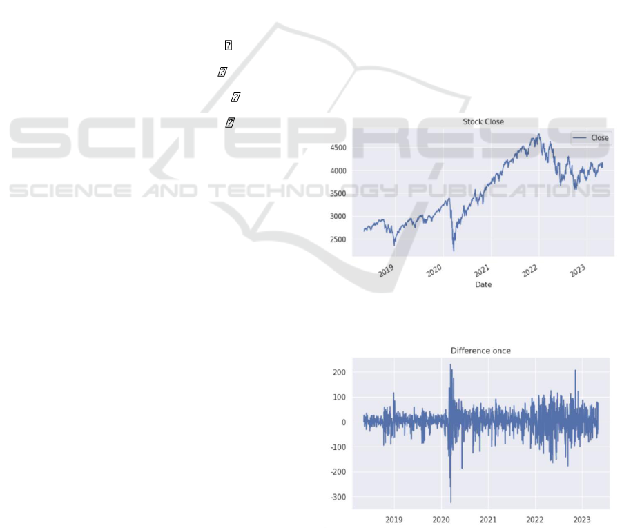
activities on the trading day (Zixia 2023). Figure 2

shows a line chart between the date and the close price

of the S&P 500 index.

b) Second Step - Check Data Stationarity: The

second step of data preprocessing involves checking

the stationarity of the data. If the data is not stationary,

a transformation such as differencing should be

performed to achieve stationary. For the ARIMA

model, the Augmented Dickey-Fuller (ADF) test is

supposed to be used to check the stationary. Because

the p-value in this case is larger than 0.05, the dataset

now is non-stationary, and differencing should be

processed. After processing the difference once, the

result in Figure 3 and 4 shows that the data has become

stationary now.

Figure 1: Close price of S&P 500 stock index for the recent

5 years (Figure credit: Original).

Figure 2: Close price data after differencing for recent 5

years. (Figure credit: Original).

DAML 2023 - International Conference on Data Analysis and Machine Learning

446

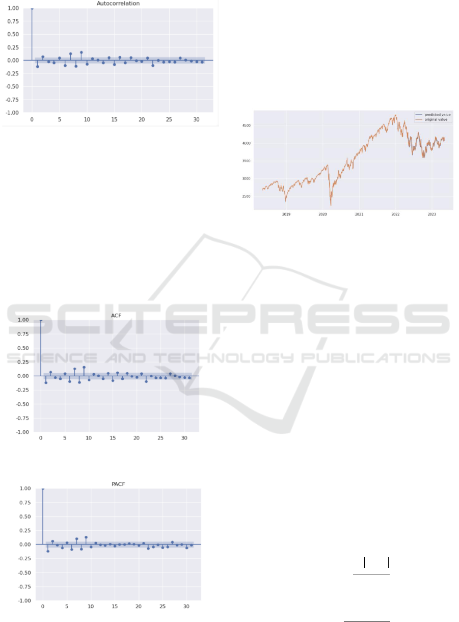
Figure 3: Autocorrelation function plot(ACF) (Figure credit:

Original).

3.1.2 Model Identification

The second step involves determining the appropriate

values for the three parameters (p, d, q) of the ARIMA

model. According to the result above, since the dataset

requires one integration to achieve stationarity, d

should be set to 1. Subsequently, the plots of the

AutoCorrelation Function (ACF) and Partial

AutoCorrelation Function (PACF) can be utilized to

identify the values of p and q, respectively. According

to the ACF plot in Figure 5 and PACF plot in Figure

6, p is proper to be 3 and q is proper to be 2.

Figure 4: Autocorrelation function plot (ACF) (Figure

credit: Original).

Figure 5: Partial AutoCorrelation function plot (PACF)

(Figure credit: Original).

3.1.3 Model Fitting and Forecasting

Next, the ARIMA (3,1,2) model is constructed,

utilizing the closing prices of the S&P 500 index from

May 7, 2018, to May 5, 2023, to train the model. Using

the fitted model, the close price of the stock index

from 2022-5-6 to 2023-5-5 is predicted. Figure 7

displays a comparison of the predicted price of the

S&P 500 index with the original price.

Figure 6: ARIMA Model predicted value vs. Original value

of Close Price (Figure credit: Original).

3.1.4 Model Evaluation

The purpose of the model evaluation is to assess the

accuracy of the model used in the prediction. There

are quite a few different metrics that can be used for

evaluating the accuracy of time series forecasting

models. This paper employs the three most common

metrics for evaluation: Mean Absolute Error (MAE),

Mean Squared Error (MSE), and Root Mean Squared

Error (RMSE). The MAE is defined as the average of

the absolute difference between predicted and actual

values, but it may be sensitive to outliers. Equation (6)

is used to express the MAE, where is the predicted

value, xi is the actual value, and the letter n represents

the total number of values in the test set. The MSE

measures the average squared difference between

predicted and actual values, and it can be expressed by

(7). The RMSE is simply the square root of the MSE,

which is shown by (8) (Lendave 2021). All three

metrics yield positive values, and a closer

approximation to 0 indicates superior model

performance. The MAE, MSE, and RMSE scores for

the ARIMA predicted model are 42.7936, 3008.1958,

and 54.8470, correspondingly.

MAE

−



(6)

( )

MSE

−



(7)

Evaluating ARIMA and LSTM Approaches for Predicting S&P 500 Index Movements: A Comparative Analysis

447

( )

RMSE

−



(8)

3.2 Procedure and Results of the LSTM

Model

After demonstrating the overall procedure and results

of using the ARIMA model to make the prediction,

here is the procedure and results of the LSTM model.

The main structure of building this model and using it

to forecast is similar to the ARIMA model, which also

contains 4 core steps, that is data preprocessing, model

building, model fitting and forecasting, and finally

model evaluation.

The first step is data preprocessing. For the LSTM

model, the original data needs to experience a more

complex processing. This paper still only utilizes the

date and the close price of the S&P 500 dataset’s

columns to make the prediction. These two columns

of data require to be normalized. The ‘Date’ column

needs to be converted into a datetime format and set

as the index of the dateframe for time-series analysis.

Then, the ‘Close’ column processes normalization,

converting the numeric values of a dataset to a

common scale. It uses the MinMaxScaler in Scikit-

Learn to scale the close price of the S&P 500 stock

index between zero and one (Adusumilli 2020).

Afterward, the LSTM models need to create

sequences for training. A sequence with length 60 is

defined, and this determines how many previous time

steps your model will consider to predict the next

stock price. Then, input sequences and corresponding

labels are created. Each input sequence is a window

into historical stock prices, and the label is the next

stock price. The data is split into training and testing

sets. Typically, training relies on 80% of the data, and

testing relies on the rest of 20%. All of the operations

above are included in the data preprocessing for the

LSTM model.

What’s next, the LSTM model can be built and fit.

One or more LSTM layers, dense layers, and dropout

layers could be added in order to build a more precise

LSTM predicting model. Then, the model can be

compiled by specifying the optimizer ‘adam’ and the

loss function—'mean_squared_error’. The model can

be trained using the training data, specifying the

number of epochs (iterations through the training data)

and the batch size (the number of samples used in each

training step). The steps in building the LSTM model

is completed. After model building and model fitting,

it uses the trained model to make predictions on the

test data, and inversely transforms the predictions to

obtain the actual stock price in the original scale. The

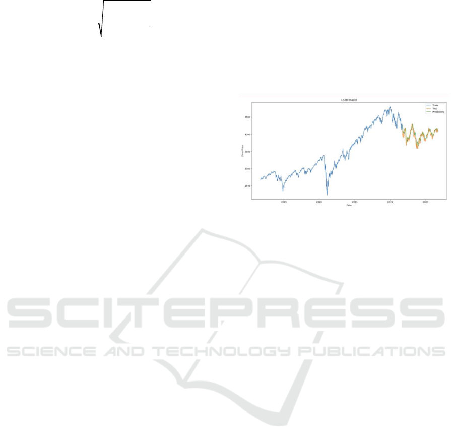
visual result of the original value and the predicted

value of the data is shown in Figure 8. Finally, the

MAE, MSE, and RMSE matrices can be used as well

to measure the accuracy of the prediction using the

LSTM model. Approximately, the result of MAE is

74.0982, the result of MSE is 9364.4735, and the

result of RMSE is 96.7702.

Figure 7: LSTM Model predicted value vs. Original value of

Close Price. (Figure credit: Original).

4 DISCUSSION

This section of the paper compares the predictive

performance of the ARIMA and LSTM models using

their respective predicted results and evaluation

metrics and based on these comparisons, the strengths

and weaknesses of each model are summarized.

To analyze the predicted results of these two

models, Figure 7 and Figure 8 are representative. The

orange line in Figure 6, and the blue and orange lines

in Figure 8 show the original close price of the S&P

500 stock index from around 2018 to 2023. While the

blue line in Figure 7 and the green line in Figure 8 are

the predicted close prices by the ARIMA model and

the LSTM model. Upon close examination of Figure

7, it is evident that the line representing predicted

values almost overlaps with the line representing

original values. There are only a few differences at the

vertices. Compared with the predicted result in Figure

7, the predicted values and the actual values in Figure

8 show more distinctions. Although the overall trend

for the predicted line and the actual line are similar,

there is little overlap between them, and the predicted

close prices are always a little bit higher than the

actual prices for the whole predicted period. In

addition, the predicted line in Figure 8 is relatively

smoother than the actual line. In other words, the

predicted line has fewer turning points than the actual

line, suggesting that it may not fully capture the

entirety of price fluctuations in the S&P 500 stock

index.

DAML 2023 - International Conference on Data Analysis and Machine Learning

448

The same conclusion can be drawn from the results

of the three error metrics. Based on the MAE, MSE,

and RMSE results for both models, it is evident that

the values of these three matrices for the ARIMA

model are lower than the LSTM model, which means

that the predicted accuracy of the ARIMA model in

this case is higher than the LSTM model. Therefore, it

is reasonable to conclude that, in the given context, the

ARIMA model outperforms the LSTM model in

predicting the stock price from the standpoint of the

predicted graphs and the assessment outcomes of

these two models.

Generally speaking, both the ARIMA model and

the LSTM model have benefits and drawbacks. The

ARIMA model offers simplicity and has a well-

defined structure. Only the parameters of the model

need to be estimated from the data. The drawback of

the ARIMA model is that the time series data needs to

be stable when used in the ARIMA model. If the data

is unstable, the ARIMA model may fail to capture the

underlying pattern and produce accurate predictions.

It is widely recognized that initial stock data are non-

stationary, necessitating certain preprocessing steps

for prediction. The LSTM model is an enhanced RNN

model that fixes issues with RNN while retaining the

majority of its characteristics. It is an ideal model for

dealing with issues that are highly correlated with time

series, like the stock prediction problem discussed in

this paper. Theoretically, by adjusting the number of

layers and several specific parameters in the LSTM

model, its predictive accuracy should be significantly

improved. However, one of the drawbacks is that the

LSTM model needs higher hardware requirements

when dealing with longer training time for running

predictions. It may take hours to run when processing

datasets over a long time span. The aforementioned

studies indicate that the lightweight LSTM model's

forecasting accuracy is actually less than that of the

ARIMA model. Additionally, these results suggest

that it is challenging to demonstrate the benefits of

LSTM in the typical network construction and

operating scenario (Wenjuan 2021).

5 CONCLUSION

This paper commences by outlining the theoretical

underpinnings of two widely used time-series models:

the ARIMA and LSTM models. Subsequently, this

paper, using the close prices of the S&P 500 stock

index in the recent 5 years as a dataset, basically states

the building process and the forecasting results of

these two models. Finally, the comparison between

the results of these two models suggests that although

in this situation the ARIMA model predicts better than

the LSTM model, both models have advantages and

disadvantages. Thus, it is important to notice that the

choice between the ARIMA and LSTM models for

stock price forecasting should be based on the specific

features of the data and the forecasting horizon. The

whole study using two of time-series models offers

guidance to investors and researchers seeking to make

informed decisions in the dynamic world of financial

markets. There are many more relative time-series

models that can be used to predict stock prices or stock

index prices, all of which warrant further investigation

and may prove beneficial for future stock price

predictions.

REFERENCES

G. Gaiwen and W. Shihan, "Stock price prediction based on

gray theory and ARIMA model," Journal of Henan

Institute of Education (Natural Science Edition), vol. 32,

no. 02, pp. 22-27, 2023.

J. Young, M. Kazel, and G. Scott, "Market Index:

Definition, How Indexing Works, Types, and

Examples," Investopedia, Jul. 23, 2023.

J. Wang, J.-Z. Wang, Z.-G. Zhang, and S.-P. Guo, "Stock

index forecasting based on a hybrid model," Omega,

vol. 40, no. 6, pp. 758-766, 2012.

W. Kenton, "Understanding S&P 500 Index – Standard &

Poor’s 500 Index," Investopedia, Mar. 23, 2021.

Tableau, "Time Series Forecasting: Definition,

Applications, and Examples," 2023/8/1, 2023/9/17,

https://www.tableau.com/learn/articles/time-series-

forecasting.

A. Garlapati, D. R. Krishna, K. Garlapati, N. m. Srikara

Yaswanth, U. Rahul and G. Narayanan, "Stock Price

Prediction Using Facebook Prophet and Arima Models,"

in 2021 6th International Conference for Convergence

in Technology (I2CT), Maharashtra, India, 2021, pp. 1-

M. Ameri, "s&p500_daily_2018-05-07 to 2023-05-05,"

Kaggle, May 2023.

https://www.kaggle.com/datasets/mojtabaameri/s-and-

p500-daily-2018-05-07-to-2023-05-05.

A. A. Ariyo, A. O. Adewumi and C. K. Ayo, "Stock Price

Prediction Using the ARIMA Model," in 2014 UKSim-

AMSS 16th International Conference on Computer

Modelling and Simulation, Cambridge, UK, pp. 106-

112, 2014.

B. Guha and G. Bandyopadhyay, "Gold Price Forecasting

Using ARIMA Model," Journal of Advance

Management Journal, 2016.

C. Haowei, "A comparative study of models related to stock

price forecasting," Chongqing University, 2023.

Z. Hanqing, "Research on stock price prediction based on

long and short-term memory neural network," Chengdu

University of Technology, 2023.

Evaluating ARIMA and LSTM Approaches for Predicting S&P 500 Index Movements: A Comparative Analysis

449

W. Zixia, "Stock price analysis and forecasting based on

ARIMA model--Construction Bank as an example,"

Modern Information Technology, vol. 7, no. 14, pp.

137-141, 2023.

V. Lendave, "A Guide to Different Evaluation Metrics for

Time Series Forecasting Models," Analytics India

Magazine, Nov. 1, 2021.

R. Adusumilli, "Predicting Stock Prices Using a Keras

LSTM Model," Medium, Jan. 29, 2020.

D. Wenjuan, "Comparison of ARIMA model, LSTM model

based on stock prediction," Industrial Control

Computer, vol. 34, no. 07, pp. 109-112+116, 2021.

DAML 2023 - International Conference on Data Analysis and Machine Learning

450