Enhancing Directional Accuracy in Stock Closing Price Value

Prediction Using a Direction-Integrated MSE Loss Function

Haojie Yin

Department of Applied Mathematics, University of California,Berkeley, Berkeley, United States

Keywords: Loss Function, LSTM, BiLSTM, Stock Price Prediction, DI-MSE, Directional Accuracy.

Abstract: In financial markets, Long Short-Term Memory (LSTM) and Bidirectional Long Short-Term Memory

(BiLSTM) models have been proved to achieve high “accuracy” in predicting the next closing price. However,

such “accuracy” is commonly referred to price value accuracy-how close the predicted and real prices are.

Many prediction models neglect the directional accuracy of predicted prices due to the natural characteristic

of Mean Square Error (MSE) as loss function. A predicted price with accurate value can potentially be in the

wrong direction which causes significant loss to investors and traders’ wealth. Instead, a useful prediction

requires both the correct direction and a value close to real prices. To achieve such a combination and improve

directional accuracy, a novel loss function Direction-Integrated Mean Square Error (DI-MSE) is introduced

by incorporating directional loss information to conventional MSE. Among 28 stocks including both single

stock and stock indices, such as Apple or SP500, DI-MSE is shown to increase the average directional

accuracy to nearly 60%. At the same time, the average value accuracy of predicted price remains around 98%.

1 INTRODUCTION

Stock price prediction has been a prominent challenge

in contemporary financial markets due to high

proficiency by stock trading. With an accurate

prediction of the next closing price in certain stocks,

investors can decide whether to sell shares or keep

their shares in order to increase their wealth. Indeed,

such a prediction requires two pieces of accurate

information: what is the value of the next closing price

and the movement’s direction of next closing price. In

other words, the stock price prediction can be divided

into two components: price value prediction and price

direction prediction. Researchers have achieved

significant success in those components: Liu achieves

around 78% accuracy on price direction (Liu et al

2018). Ding’s associated network model of Long

Short-Term Memory can predict multiple price value

at the same time with 95% accuracy (Ding and Qin

2022). And Roondiwala minimizes the testing Root

Mean Square Error (RMSE) to 0.00859 when

predicting price value for stock NIFTY 50

(Roondiwala et al 2017). In fact, those two individual

components are always done distinctly: while the

direction predictions concentrate on solely predicting

a correct direction without predicting a price value, the

price value predictions focus on minimize the residual

between predicted and true values without considering

the correctness of the prediction’s direction. Such lack

of consideration on direction is the main disadvantage

of Mean Square Error (MSE), a common loss function

used for model training. By training with MSE, a

model may predict prices with high accurate value but

instead in the wrong direction, which causes loss of

investors. This is the primary challenge faced by price

value prediction: poor directional accuracy. This

paper introduces a novel loss function, Direction-

Integrated Mean Square Error (DI-MSE), as a try to

address such a challenge.

A few researchers also implemented specific loss

function to enhance the performance of prediction on

stock related fields. For example, Dessian

implemented a custom loss function which computed

loss of predicted value depending on its directional

correctness to improve the prediction of assets returns

(Dessain 2022). Moreover, Yun designed a joint lost

function which takes account of the direction of return

in certain periods to improve the prediction

performance on maximize the return in asset portfolio

(Yun et al 2020). Zhou also introduced directional

error to improve value predictions in Generative

Adversarial Nets algorithm (Zhou et al 2018). For

stock price predictions, Doshi noticed the poor

directional accuracy for models trained by MSE and

designed a custom loss function by assigning different

weights based on directional correctness (Doshi et al

2020). However, some of those custom loss functions

Yin, H.

Enhancing Directional Accuracy in Stock Closing Price Value Prediction Using a Direction-Integrated MSE Loss Function.

DOI: 10.5220/0012810200003885

Paper published under CC license (CC BY-NC-ND 4.0)

In Proceedings of the 1st International Conference on Data Analysis and Machine Learning (DAML 2023), pages 119-126

ISBN: 978-989-758-705-4

119

are difficult to generalize predicting next closing price

in more stocks.

DI-MSE, on the other hand, goes beyond MSE.

While calculating how close the predicted value and

true values are like MSE, DI-MSE incorporates the

directional information by computing the directional

loss of predicted values, considering the correctness of

directions but also the proportion of specific direction

in real prices. DI-MSE dynamically adjusts its focus

during the training process, automatically transiting

from directional correctness to price value accuracy.

As an expanded version of MSE, DI-MSE aims to

minimize both the number of wrong directions and the

difference between predicted and true values.

Consequently, DI-MSE assists models in training to

predict accurate closing prices with enhanced

directional accuracy.

In this paper, a detailed construction of DI-MSE

will be introduced, followed by the methodology of

experiments and analysis of the results to compare

usage of MSE and DI-MSE in model training for price

value predictions.

2 PROBLEM DESCRIPTION

By using MSE, models are trained by minimizing the

marginal between predicted and real value in prices.

However, those models can hardly learn to predict the

correct direction during training process, as MSE

provides no directional information for training.

Under such circumstances, the trained model tends to

gain high accuracy of predicting closing price but poor

directional accuracy. Consider an example: on a

particular day, stock A has a closing price of 125

dollars. The next closing price predicted by two

distinct models is 120 and 140 dollars, and the real

next closing price is 130 dollars. By computing price

accuracy (PA) defined by:

PA = (1 — | — y|/y) × 100%, ()

where  represents predicted price and y represents

real price, it can be noticed that the price accuracies of

two predictions are the same:

|120 130 |

1 100% 92.3%,125 120(down direction)

130

|140 130 |

1 100% 92.3%,125 140(up direction)

130

−



−   





 



−





−   









()

However, the directions of both predictions are

rather opposite. Compared to the current latest closing

price of 125 dollars, the real next closing price of 130

dollars shows an increasing trend. The prediction of

140 dollars also indicates the same increasing trend,

which is indeed a “correct” direction. Conversely, the

prediction of 120 dollars indicates a decreasing trend

in “wrong” direction. For investing stock, both the

value and direction of the next closing price are

significant, as the direction is the decisive element of

selling or buying stock shares. Although one

prediction of price has a value accuracy of 92.3%, its

wrong direction may directly cause the loss of

investors. More precisely, the correctness of direction

of a prediction 

is defined by the following:

( )( )

1, 0

0, lse

i i i i

y y y y

−−



− − 





()

where:

represents the real closing price at time i.

i-1

represents the real closing price at time i—1.



represents the predicted closing price at time i.

While D

=1 indicates a correct direction, D

indicates a wrong direction. The model trained by

MSE is likely to have prediction with wrong directions

like the example above, because MSE solely focus on

minimizing the marginal between 

and y

without

considering if the direction is correct or not. To

enhance the model’s capability of predicting a closing

price close to real value, more importantly, with a

correct direction, MSE requires additional directional

information during model training.

3 NEW LOSS FUNCTION:

DIRECTION-INTEGRATED

MEAN SQUARE ERROR

(DI-MSE)

One widely used loss function for predicting stock

prices is Mean Square Error (MSE). Given predicted

value set y

pred

and real value set y

real

, MSE computes

total error by:

( )

MSE y y

=  −

()

where:

represents the real closing price at time i.



represents the predicted closing price at time i.

n represents the size of y

pred

However, MSE only considering the marginal

difference between y

and 

at same time point i

without distinguishing the directions. To address such

limitations, Direction-Integrated mean square error

(DI-MSE) is introduced. DI-MSE is decomposed into

two distinct parts based on the directional correctness

of predictions by (5):

DAML 2023 - International Conference on Data Analysis and Machine Learning

120

DI-MSE = DLC + DLW ()

where:

DLC represents the total directional loss for all 

with correct direction (D

=1) by (3).

DLW represents the total directional loss for all 

with wrong direction (D

=0) by (3).

Similar to traditional MSE, DLC is computed by

averaging of squared errors of all 

. Differently, DLC

is computed by only 

with the correct direction and

weights those square errors based on the percentage of

corresponding direction in y

real

. The directional weight

is computed using (6):

( )

100%,

−











−













−



()

where:

represents the price value in time k.

I (y

≥ y

k-1

) represents an indicator function

outputting value of 1 if the condition y

≥ y

k-1

is true

otherwise 0.

Notably, since there is no preceding real closing

price y

available for comparison before the first real

closing price y

in y

real

, it is impossible to ascertain the

directional correctness of 

. As a result, the loss for 

is set to 0 to avoid adverse effect on loss computation

due to an unknown real direction. Consequently, the

summation begins from i=2 in (6). With directional

weights in (6), DLC is computed by (7):

( )

i i i

DLC W y y



=−













()

where n’ denoting the number of predictions with the

correct direction. If the directions in a batch of training

data is mainly upward, it can be referring as closing

price keeps increasing in this period. (This is

guaranteed by that the training set is in time order and

model structure divide batches also in time order)

With the premise that predictions have correct

directions, the predictions with upward direction are

weighted more heavily, help the model to further

follow the overall increasing trend. DLC is responsible

for helping models predict closing prices closer to real

value.

On the other hand, DLW is responsible for helping

models predict a closing price with the correct

direction. By counting the number of predictions with

wrong direction, DLW is computed by

DLW

=

 ()

By (7) and (8), the computation of DI-MSE in (5)

can be reformulated into:

( )

- 1.

i i i

DI MSE W y y



=  − + 









()

After the normalization step, all real closing

prices, as long as output value, are all in range of [0,

1]. With W

, as a percentage in range of [0, 1], the

individual error W

(

—y

)

for predictions with

correct direction will be small compared to 1, the error

for predictions with wrong direction. Such difference

prompts the model to learn that predicting a value with

correct direction is much more beneficial to minimize

the loss function. So the model will initially focus on

predicting correct directions. When the training

progresses, the less predicted values have wrong

directions so that more predicted values have their loss

computed in DLC of (7) instead of DLW of (8). In this

case, the focus of DI-MSE transits from the directional

correctness to the accuracy of predicted values. In fact,

when all predictions are with correct directions, DLW

equals 0 thus DI-MSE is only composed of DLC,

almost the same as MSE except for the directional

weight. Under such circumstances, DI-MSE fully

focuses on price value accuracy. When combining

DLC and DLW, DI-MSE can provide how accurate the

predicted values are and how correct the predicted

values’ directions are. With incorporated directional

information, DI-MSE is expected to help models

improve the directional accuracy on predictions.

4 DESIGN METHODOLOGY

4.1 Dataset

To demonstrate the generalization of modified loss

function across different stocks, the dataset contains

historical data of 20 single stocks and 8 stock indices,

in time order from 2015-09-02 to 2023-08-14. A

detailed list of all included stocks is presented in

TABLE I. In the dataset, each stock is presented with

2000 data points. Each data point contains 6 distinct

feature values: Open price, High price, Low price,

Close price, Volume, and 30-Day ROC. At certain

timestep n, the feature of 30-Day Rate of Change

ROC

is computed by the formula:

ROC

= (Close

— Close

n—30

) / Close

n—30

, ()

Enhancing Directional Accuracy in Stock Closing Price Value Prediction Using a Direction-Integrated MSE Loss Function

121

where:

represents the Closing price at timestep n.

n—30

represents the Closing price at timestep

n—30, which is the Closing price from 30 trade days

in the past.

Table 1: Stock Lists in Dataset.

Single

Stocks

AAPL, MSFT, AMZN, META, TSLA, SPY,

GOOGL, GOOG, BRK-B, JNJ, JPM, NVDA, V,

DIS, PG, UNH, MA, BAC, NFLX, QQQ

Stock

Indices

000001.ss, 399001.sz, ^HSCE, ^HSCC, ^GSPC,

^DJI, ^IXIC, ^SP500-20

While the Close Price is set as the output feature to

be predicted, all features including Closing price are

set as the input features for model input.

4.2 Data Preprocessing

In data preprocessing phase, several steps were

implemented to prepare the data for model training

according to the objective of predicting the next

closing price by utilizing data of the past 30 trade days.

Initially, the first 1870 data points in the dataset are set

as the training set and the 130 data points left are set

as testing set. Particularly, the splitting was based on

timestep, and the testing set contained the most recent

130 data points. Consequently, predicted results of the

testing set directly demonstrated the predictability of

model in newest stock price trend.

To avoid the potential bias effect due to scale

difference among feature values, such as Volume and

Close Price, a rescaling process was applied to ensure

the uniformity within dataset. Such a process

transformed all feature columns, in both training and

testing set, into a consistent range of [0,1]. For each

feature, the original value x

in time i was transformed

i_normalized

= (x

— min

) / (max

— min

), ()

where:

i_normalized

represents the normalized value of x

min

represents the minimum value among feature

values in training set.

max

represents the maximum value among feature

values in training set.

It is essential to underscore that normalization

process applied to testing set adheres to the minimum

and maximum values derived from the training set.

This approach prevented the potential data leaking

from future values in the testing set. If normalization

in testing set utilize minimum and maximum values

derived from the testing set itself, the normalized data

will obtain the information for future data and

diminish the effectiveness of evaluating testing set

results.

Next, both the training set and testing set were

processed by time sequence transform with timestep

of 30. For any closing price y

at time i, the input data

was constructed by the preceding 30 data points,

ranging from x

i-1

to x

i—30

. Each x contained 6 feature

values. In other words, this step constructed the data

into format such that the model inputs the data of past

30 days and predicts the next closing price. After

finishing all data processing, the datasets obtained

dimensions listed in TABLE II.

4.3 Model Architecture

Mootha’s and Shah’s research showed Long Short-

Term Memory (LSTM) and Bidirectional Long Short-

Term Memory (BiLSTM) models obtained a good fit

for price value predictions with low RMSE (Mootha

et al 2020 & Shah et al 2021). Thus, LSTM and

BiLSTM were used for validating the efficiency of DI-

MSE in this study as well. As Sunny’s research on

hyperparameter tunning suggested that fewer number

of layers in LSTM and BiLSTM algorithm is likely to

improve the model fitting, one layer was applied in

constructing the following model architectures (Sunny

et al 2020).

LSTM Architecture: the LSTM model structure

comprises a single LSTM layer with 200 units. To

prevent potential overfitting, a L2 regularization with

a strength of 1×10

—6

is applied within the LSTM

layer. The following layer is a dropout layer using 0.3

dropout rate. The structure ends with a single dense

layer. The training set is divided into batches of 32 and

processes 200 epochs of training based on the Adam

optimizer.

BiLSTM Architecture: the BiLSTM model

structure comprises a single BiLSTM layer. The

BiLSTM layer is built by one forward LSTM layer

and one backward LSTM layer. Both LSTM layers are

consisted with 200 units and applied with a L2

regularization with a strength of 1×10

—6

. There is a

dropout layer using 0.3 dropout rate after the BiLSTM

layer. This structure ends with a single dense layer.

The training set also is divided into batches of 32 and

processes 200 epochs of training based on the Adam

optimizer.

4.4 Validation Procedure

For each stock in the dataset, the validation procedure

followed these steps:

1) With the training set, utilized the LSTM

Architecture to train two models: one using MSE as

loss function and one using DI-MSE as loss function.

DAML 2023 - International Conference on Data Analysis and Machine Learning

122

2) With the testing set, predicted two groups of

outputs 

from the two models. As the outputs were

normalized, they were inversely transformed back to

price values 

i_unnormalized

using the minimum min and

maximum max of the closing price feature in the

training set:



i_unnormalized

= 

× (max — min) + min. ()

Table 2: Dimensions of Training and Testing Dataset.

Training Set Input

1840×30×6

Training Set Output

1840×1

Testing Set Input

100×30×6

Testing Set Output

100×1

3) Compared two models’ performance on their

predicted closing prices.

4) Repeated steps 1-3 with BiLSTM Architecture

4.5 Validation Metrics

For comparison in each stock, two metrics were

applied for evaluating the predictions in the testing set:

mean price accuracy (MPA) and directional accuracy

(DA). Using the definition of PA in (1), MPA is

computed by

1 100%,

MPA



−



=  − 





()

where:

n represents the size of the testing set.

represents the real closing price at time i.



represents the predicted closing price at time i.

A high MPA indicates a small difference between

the predicted and the real closing price. While MPA

evaluates averagely how accurate the predictions are,

DA evaluate how correct the predictions’ direction is,

by the following formula:

100%,

DA D

=  

−

()

where D

indicates the direction correctness of

prediction 

as described in (3).

5 RESULT AND ANALYSIS

As shown in Figure 1 and Figure 2, DI-MSE had a

positive impact on directional accuracy DA for most

stocks in both LSTM and BiLSTM models. On

average, the use of DI-MSE in LSTM models

improved a stock’s DA from 52.96% to 60.03%.

Notably, the HSCE stock had a remarkable

improvement of 16% in DA. Similarly, BiLSTM

models trained by DI-MSE show an average increase

from 52.96% to 59.6% in DA. In other words,

compared to MSE, LSTM and BiLSTM models

trained by DI-MSE had an approximate 7%

improvement in DA. This difference in DA indicates

that DI-MSE is effective to help models predict

closing price with more correct direction.

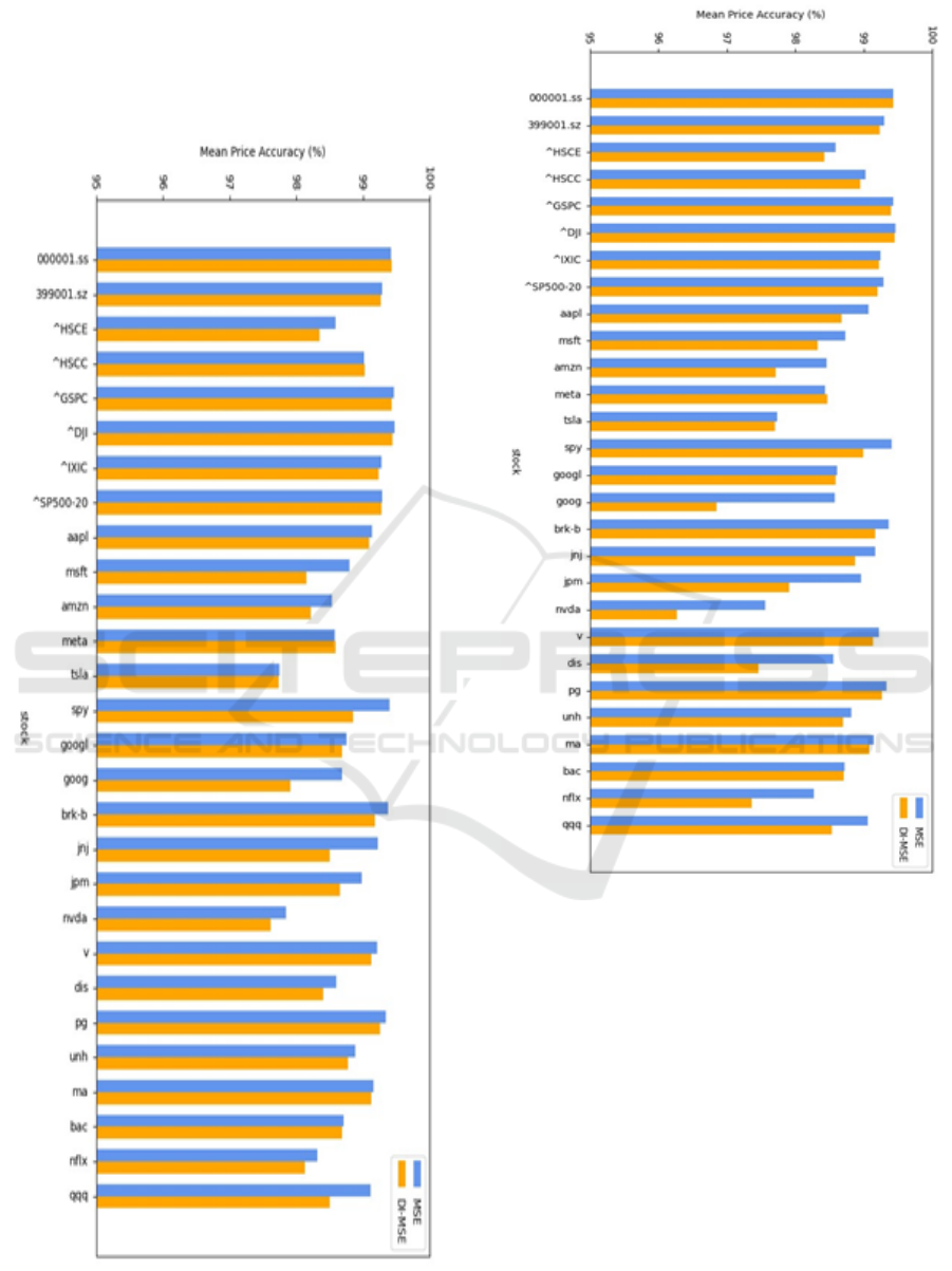
On the other hand, Figure 3 and Figure 4 show a

slight reduction in mean price accuracy MPA among

most stocks in both LSTM and BiLSTM models when

DI-MSE is applied. LSTM models trained with DI-

MSE have an average decrease in MPA of 0.2%, while

BiLSTM models trained by DI-MSE have an average

decrease of 0.35%. Because such a decrease

consistently appeared in most test stocks, it is not a

coincidence, but an effect from DI-MSE. In essence,

the application of DI-MSE as a loss function tends to

result in a decrease in value accuracy of the predicted

prices.

After replacing MSE with DI-MSE, an increased

DA but a slightly decreased MPA is observed as

mentioned above. This trade-off may be attributed to

the characteristics of DI-MSE. For predictions with

wrong direction, DI-MSE computes their losses by

DLW in (8), which does not consider the difference

between 

and y

. This lack of information in

difference potentially limits the models’ ability to

learn and predict the closing prices closer to real

values. By construction of DI-MSE, DLW plays a

crucial role in providing directional information and

determining the focus of loss function. This feature of

DI-MSE helps the models to predict closing price with

more accurate directions and then improve DA.

Consequently, DI-MSE prioritizes higher DA at the

expense of MPA, resulting in the trade-off observed in

results.

Enhancing Directional Accuracy in Stock Closing Price Value Prediction Using a Direction-Integrated MSE Loss Function

123

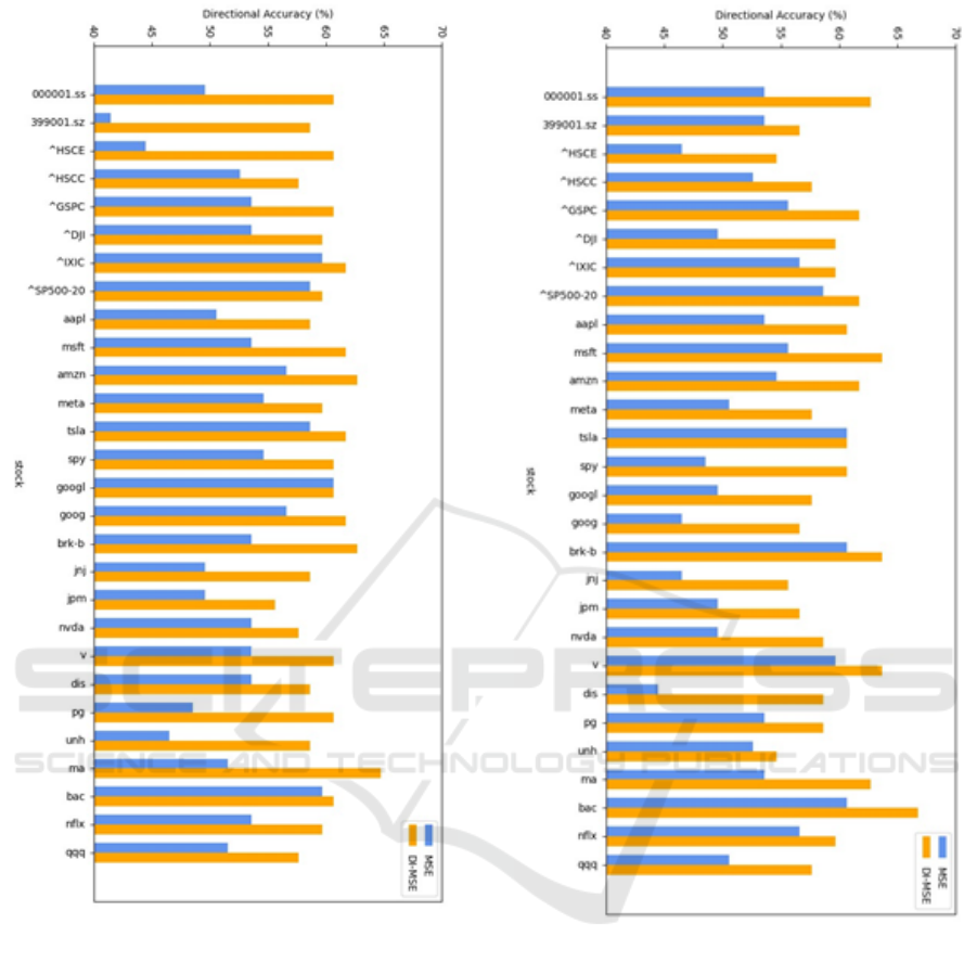
Figure 1: Comparison of DA in LSTM models trained by

MSE and DI-MSE. (Picture credit: Original).

Theoretically, DI-MSE will fully focus on

improving DA after every prediction has correct

direction. However, this case is too difficult to appear

so that DLW will inevitably exist and DI-MSE will

neglect the value accuracy on points with wrong

direction. Thus, the trade-off remains.

Figure 2: Comparison of DA in BiLSTM models trained by

MSE and DI-MSE. (Picture credit: Original).

In another aspect, current input from training data

maintains the time order without shuffle. Shuffling the

training data (after time-sequence transforming) can

possibly help the model to further generalize the price

pattern and give a more accurate prediction. However,

if a model struggles to decrease the number of

predictions with wrong predictions, the focus of

training will stay at directional correctness and neglect

to increase the price value accuracy. This model may

end up with poor accuracy in both direction and value,

as a potential limit of DI-MSE. One possible

improvement is to modify the error value for wrong

direction in DLW or (8). DI-MSE adjusts the focus by

DAML 2023 - International Conference on Data Analysis and Machine Learning

124

considering the difference of error magnitude in

direction correctness. By modifying DLW, such

difference can be enlarged or diminished and change

the degree of priority on directional accuracy in DI-

MSE.

Figure 3: Comparison of MPA in LSTM models trained by

MSE and DI-MSE. (Picture credit: Original).

Figure 4: Comparison of MPA in BiLSTM models trained

by MSE and DI-MSE. (Picture credit: Original).

6 CONCLUSION

In both LSTM and BiLSTM models, by applying DI-

MSE, the price value accuracy (the average of MPA

in all stocks) has a diminutive decrease of 0.2% and

0.35%, respectively. However, in exchange, the mean

of directional accuracy in test stocks has an increase

of nearly 7% compared to using MSE. The result

demonstrates that DI-MSE can promote the

directional accuracy of predictions up to nearly 60%,

while maintaining nearly same price value accuracy.

With such directional accuracy, it is proved that the

models trained by DI-MSE have predictability on

direction instead of solely following the past

Enhancing Directional Accuracy in Stock Closing Price Value Prediction Using a Direction-Integrated MSE Loss Function

125

directions or randomly guessing. To a certain degree,

the combination of price value and directional

prediction is achieved by DI-MSE.

Based on the validation, the results show LSTM

and BiLSTM models trained by DI-MSE can make

prediction of next closing price in average nearly 98%

value accuracy and nearly 60% directional accuracy.

With such predictions, the investors are able to make

more appropriate decisions and earn more profits.

DI-MSE has shown an enhancement in the LSTM

and BiLSTM, two fundamental algorithms for price

value predictions. By generalizing and applying DI-

MSE in more advanced algorithms derived from

LSTM, the models may achieve better value and

directional accuracy among predictions. In addition,

DI-MSE can be further generalized to all machine

learning problems in various fields which consider

accuracy of both value and direction, such as future

temperature or humidity. In a novel path for machine

learning, more custom loss functions will appear for

various model training tasks.

REFERENCES

S. Liu, G. Liao and Y. Ding, “Stock transaction prediction

modeling and analysis based on LSTM,” 2018 13th

IEEE Conference on Industrial Electronics and

Applications (ICIEA), Wuhan, China, 2018, pp. 2787–

2790.

Ding, G., Qin, L. “Study on the prediction of stock price

based on the associated network model of LSTM,”

International Journal of Machine Learning and

Cybernetics, 2022, vol. 11, pp. 1307–1317.

M. Roondiwala, H. Patel, and S. Varma, “Predicting Stock

Prices Using LSTM,” International Journal of Science

and Research (IJSR), 2017, vol. 6, pp. 04.

J. Dessain, “Improving the prediction of asset returns with

machine learning by using a custom loss function,”

SSRN Electronic Journal, 2022.

H. Yun, M. Lee, Y. S. Kang, and J. Seok, “Portfolio

management via two-stage deep learning with a joint

cost,” Expert Systems with Applications, 2020, vol.

143, pp. 113041.

X. Zhou, Z. Pan, G. Hu, S. Tang, and C. Zhao, “Stock

market prediction on high-frequency data using

generative adversarial nets,” Mathematical Problems in

Engineering, 2018, pp. 1–11.

A. S. Doshi, A. Issa, P. Sachdeva, S. Rafati, and S. Rakshit,

“Deep Stock Predictions,” ArXiv, vol. abs/2006.04992,

2020, unpublished.

S. Mootha, S. Sridhar, R. Seetharaman and S. Chitrakala,

“Stock Price Prediction using Bi-Directional LSTM

based Sequence to Sequence Modeling and Multitask

Learning,” 2020 11th IEEE Annual Ubiquitous

Computing, Electronics & Mobile Communication

Conference (UEMCON), New York, NY, USA, 2020,

pp. 0078–0086.

J. Shah, R. Jain, V. Jolly and A. Godbole, “Stock Market

Prediction using Bi-Directional LSTM,” 2021

International Conference on Communication

information and Computing Technology (ICCICT),

Mumbai, India, 2021, pp. 1–5.

M. A. Istiake Sunny, M. M. S. Maswood and A. G. Alharbi,

“Deep Learning-Based Stock Price Prediction Using

LSTM and Bi-Directional LSTM Model,” 2020 2nd

Novel Intelligent and Leading Emerging Sciences

Conference (NILES), Giza, Egypt, 2020, pp. 87–92.

DAML 2023 - International Conference on Data Analysis and Machine Learning

126