Forecasting Nasdaq Price Index: A Comparative Study of Regression

and Time Series Analysis

Ziheng Li

Department of Math, Franklin and Marshall College, Lancaster, U.S.

Keywords: Forecasting, ARIMA, Linear Regression, Cubic Spline Regression, Seasonality.

Abstract: The Nasdaq Stock Market, one of the world's premier stock exchanges, serves as an imperative indicator of

economic activity and investor sentiment. Accurate forecasting of the Nasdaq Price is of paramount

importance for a myriad of stakeholders, ranging from policymakers to individual investors. This study

embarks on an exhaustive journey to discern the most efficacious forecasting method for this critical indicator.

We systematically compare the predictive prowess of several techniques: the (Autoregressive Integrated

Moving Average) ARIMA models, linear regression, cubic spline regression, and a decomposition approach

that identifies and leverages underlying trends and seasonality. The culmination of our rigorous analyses

revealed that the cubic spline regression outperformed the other contenders, marking itself as the most apt

model for forecasting the Nasdaq Price within the scope of this study if without any significant and unexpected

events. This article provides an analysis of various forecasting methods for predicting the Nasdaq Price. The

article compares the predictive accuracy of different techniques, including ARIMA models, linear regression,

cubic spline regression, and a decomposition approach that identifies and leverages underlying trends and

seasonality. This article provides valuable insights into effective forecasting methods for economic indicators

and investor sentiment.

1 INTRODUCTION

The NASDAQ index, as a quintessential

representative of the technology sector, occupies an

influential position within the global financial

landscape. A blend of nascent startups and tech

behemoths, NASDAQ acts not just as a gauge of the

technology industry, but also provides indications of

economic trends and market sentiments. Its intricate

dance of rises and falls, often seen as an embodiment

of the tech world's vitality, requires meticulous

understanding (Schwert 1990).

Being tech-centric sets the NASDAQ Composite

apart. Unlike broader market indices such as the S&P

500 or the Dow Jones Industrial Average, which

encompass a more extensive range of sectors,

NASDAQ predominantly mirrors the tech sector's

dynamism in the U.S. stock market. Consequently,

the volatility often associated with tech innovations,

regulatory shifts, and international trade relations

becomes more pronounced in this index (Fama and

French 1993). Financial market dynamics are ever

evolving. Traditional time-series forecasting models,

although valuable, have started to mingle with

innovative, data-driven paradigms. The emergence of

machine learning, especially, has reshaped the art of

financial forecasting. From being limited to linear

regression models and Autoregressive Integrated

Moving Average (ARIMA), researchers have started

to embrace complex architectures like neural

networks and support vector machines. These tools,

with their capacity to handle vast datasets and discern

patterns, offer tantalizing prospects for capturing the

intricate, nonlinear dynamics inherent in stock

markets (Kim 2003).

The ramifications of macroeconomic indicators

on stock indices can't be emphasized enough. GDP,

interest rates, unemployment rates, among others, have

traditionally been viewed as beacons that shed light on

an economy's health. For indices like NASDAQ, these

indicators are not just abstract numbers but pivotal

drivers. The ebb and flow of the tech sector, influenced

by these economic indicators, can lead to profound

implications for investors, policymakers, and

stakeholders (Chen and Ross 1986).

A pertinent question arises with the multitude of

factors influencing the NASDAQ, how does one

distill the essential from the noise. Global events,

from trade wars to pandemics, have shown their

potential to cause significant market upheavals. The

Li, Z.

Forecasting Nasdaq Price Index: A Comparative Study of Regression and Time Series Analysis.

DOI: 10.5220/0012814400003885

Paper published under CC license (CC BY-NC-ND 4.0)

In Proceedings of the 1st International Conference on Data Analysis and Machine Learning (DAML 2023), pages 515-521

ISBN: 978-989-758-705-4

515

tech sector, given its global interconnectedness,

remains especially vulnerable. This necessitates

comprehensive models that encapsulate not just

economic data but also global sentiments, news

trends, and geopolitical shifts (Tetlock 2007).

Moreover, understanding NASDAQ's behavior

is not just for short-term trading benefits. Long-term

investors, regulators, and even governments have

stakes in its trajectory. For institutional investors,

predictive insights can guide strategic asset

allocation. Regulators, wary of market bubbles and

potential crashes, can benefit from early warning

systems. Governments, especially those aiming to

foster tech innovation, can gauge investor sentiments

and tweak policies accordingly (Baker and Wurgler

2007). The reliance on technology and its evolving

nature has meant that the NASDAQ index is not

merely influenced by traditional financial metrics.

The realm of technology is vast, and factors like cyber

threats, technological breakthroughs, and even digital

currency fluctuations have started to find their footing

as potential influencers on the NASDAQ trajectory

(Nasdaq composite index 2023).

Further, with the emergence of green

technologies and the increasing importance of

sustainable practices in the tech sector, ESG

(Environmental, Social, and Governance) factors

have also begun to cast an influence on NASDAQ's

movements. Companies listed on the NASDAQ,

especially those deeply involved in tech innovations,

are under scrutiny for their ESG compliance, and this

has potential ramifications for their stock

performance and, by extension, the NASDAQ index

(Nadaq Price 2023).

This research, therefore, is more than an

academic endeavor. At its core, it's a quest to

comprehend a dynamic, multifaceted entity – the

NASDAQ. By diving deep into its historical trends,

juxtaposing it with macroeconomic indicators, and

harnessing the power of contemporary forecasting

models. Aiming to illuminate the path the NASDAQ

might traverse in the foreseeable future.

2 METHODOLOGY

2.1 Data Resources

The Nasdaq Index and Nasdaq Price (1985-2023) are

collected in (Federal Reserve Economic Data) FRED

(Nasdaq composite index 2023) and Yahoo Finance

(Nadaq Price 2023), respectively.

2.2 Method Introduction

The project used a variety of methods of forecast this

indicator using Autoregressive Integrated Moving

Average (ARIMA) models, linear regression, cubic

spline regression, trend and seasonality decomposition

techniques.

3 RESULTS AND DISCUSSION

In Figure 1 the Nasdaq Price over time graph, the

historical trend of the Nasdaq index showed long-term

upward trajectory, with periods of volatility. The

growth has been especially pronounced in the past two

decades. However, the plot also reveals certain

downturns, most notably during the economic

recessions, such as the dot-com bubble burst and the

financial crisis of 2008. We may notice that this series

may contain some non-stationarity, this can be further

verified using some graphical methods, such as ACF

and PACF, and statistical test. This will be formally

conducted in the next section. In US Monthly M2

graph, the trend for the M2 money supply

demonstrates a consistent and almost unbroken

increase over time. This rise signifies an expanding

monetary base, typically reflect a growing money

supply.

Figure 1: Correlation among Stock, M2, Interest Rate and

Unemployment Rate (Picture credit: Original).

In Figure 1, The trend in interest rates graph has

been predominantly downward, marked by periods of

volatility. This decline in rates is often a byproduct of

various central bank policies aimed at stimulating

economic growth. However, it is crucial to note that

the landscape changed dramatically after 2020, when

the covid-19 pandemic swept across the world. In

macro-economics, the interest rate generally has a

negative correlation with the stock price.

The unemployment rate graph has generally

floated around the 4-5% range, showing a stable job

market for an extended period. However, the stability

DAML 2023 - International Conference on Data Analysis and Machine Learning

516

was abruptly upended in 2020 due to the covid-19, as

a result, the rate spiked dramatically to around 12%

and decreased quickly back to 4%.

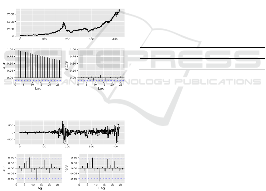
3.1 Checking ACF And PACF

Before fitting and ARIMA model, it’s essential to

check the time series data for stationarity. Using the

Autocorrelation Function (ACF) and Partial

Autocorrelation Function (PACF) plots as visualized

check, also use the Box-Pierce test as statistical test.

The ACF plot gives us an idea about the correlation

between the time series and its lagged values. The

PACF plot shows the correlation of the time series

with its lagged values that is not explained by previous

lags. Further, checking for ACF and PACF also helps

us to identify the ‘p’ and ‘q’ parameters of the ARIMA

model, which signify the order of the autoregressive

and moving average parts, respectively.

Figure 1: Original Nasdaq ARIMA Model (Picture credit:

Original).

Figure 3: First-Order Differencing ARIMA Model (Picture

credit: Original).

In Figure 2, the ACF plot displayed a characteristic

indicative of a non-stationary time series: the ACF

values did not quickly drop off towards zero, but

rather showed a gradual decline. This pattern is a

significance of non-stationarity and suggests that

differencing the series is likely required to make it

stationary for modelling. On the other hand, the PACF

plot presented a sharp drop-off after the first lag. This

immediate drop is indicative of an AR(1) process,

which suggests that only the first lag is significantly

correlated with the time series, after accounting for the

effects of the other lags. These observations from the

ACF and PACF plots guide us toward an initial

ARIMA model with differencing and a first-order

autoregressive component. In Figure 3, the ACF

displayed a rapid decay towards zero, indicating that

the differenced series has now achieved stationarity. It

also confirms the ‘I’ component in ARIMA as 1,

highlighting the need for one order of differencing to

induce stationarity. This result confirmed our

approach and shows that an ARIMA (1,1,0) may be a

potential choice.

3.2 Check Stationary

Next, Using the statistical test Box-Pierce test to test

if the original non-differencing and 1st order

differencing series are stationary. The null hypothesis

is that the series is stationary (Table 1).

Table 1: ARIMA Model Table.

X -

Squared

Degree of

Freedom

P -

vlaue

ARIMA Model

403.92

2.2e-16

(1,1,0) ARIMA

0.053898

0.8164

From the above results we can see that the results

are not surprising, showing that the original non-

differencing series is non-stationary, and after taking

differencing, the p-value of the Box-Pierce test is

0.8164, indicating the null hypothesis cannot be

rejected. Therefore, this further confirms the

reasonableness of using the (1,1,0) ARIMA model.

3.3 Fitting ARIMA Model

Finally, the auto.arima() function is used, in order to

auto select a best model using the AIC as model

selection criterion and compare the selected best

model with the (1,1,0). The auto.arima model selected

a model with (0,2,1). By observing the trace of the

selection process, the second order differencing and

compared different models and finally returned the

(0,2,1) model.

Forecasting Nasdaq Price Index: A Comparative Study of Regression and Time Series Analysis

517

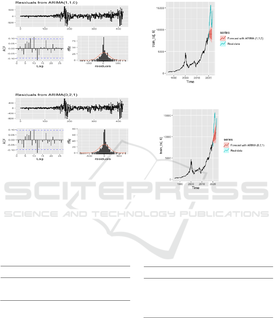
Figure 4: Residuals From ARIMA (1,1,0) (Picture credit:

Original).

Figure 2: Residuals from ARIMA (0,2,1) (Picture credit:

Original).

From the residual analysis plots we can see that the

residuals of both two models shows a stationary

residual (Figure 4 and 5). And their distribution also

looks very similar. However, the central parts of both

the histograms are far higher than the normal

distribution. This indicating a heavy center and light

tail distribution rather than normal distribution. Using

the Ljung-Box results, we can see that both residuals

are stationary (table 2).

Table 2: ARIMA Model Table.

X-squared

Degree of

Freedom

p-value

ARIMA

(1,1,0)

0.08862

0.7659

ARIMA

(0,2,1)

0.36613

0.5451

3.4 Forecasting Using ARIMA Model

The results reveal that the ARIMA (1,1,0) model

forecasts a stable, somewhat horizontal future for the

Nasdaq index. In contrast, the ARIMA (0,2,1) model

projects an upward trend for the Nasdaq index, which

aligns more closely with recent market behavior

(Figure 6, 7).

Figure 6: Forecast ARIMA Model (1,1,0) (Picture credit:

Original)

Figure 7: Forecast ARIMA Model (0,2,1) (Picture credit:

Original).

3.5 Multiple Linear Regression

Next, the multiple linear regression investigates the

correlation between the dependent variable and the

independent variables above.

Table 3: Correlation Coefficients.

Estimate

Std.

Error

t value

Pr(>|t|)

Intercept

7625.15

225.10

33.874

<2e-16

M2 Rate

-460.51

165.55

-2.782

0.00565

Interest Rate

1092.89

38.19

28.619

<2e-16

CPI Rate

33.71

219.48

0.154

0.87799

Unemployment

Rate

-840.85

50.09

16.786

<2e-16

The model explains approximately 70.19% of the

variance in the Nasdaq index, as indicated by the R-

squared value of 0.7019. Further, the coefficient of M2

rate is -460.51 with a p-value of 0.00565, indicating

that it is statistically significant at the 0.01 level (table

3). This suggests that as the M2 money supply rate

increases, the Nasdaq index decreases. The coefficient

estimate of interest rate is -1092.89 and is also

DAML 2023 - International Conference on Data Analysis and Machine Learning

518

statistically significant with a p-value close to zero.

This indicates a strong negative relationship between

interest rates and the Nasdaq index, suggesting that

when interest rate go up, the Nasdaq index goes down.

The coefficient of CPI rate is 33.71 with a p-value of

0.87799, which is not statistically significant. This

means we fail to reject the null hypothesis for the

coefficient of CPI rate being zero, implying it might

not be a good predictor for the Nasdaq index in this

model. Finally, the coefficient of the unemployment

rate is -840.85, which is statistically significant with a

p-value close to zero. This suggests a negative

correlation between unemployment rates and the

Nasdaq Index.

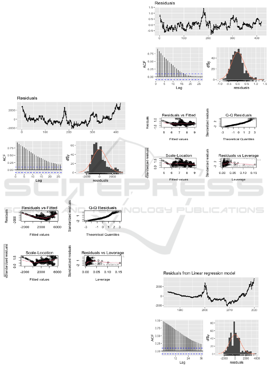
Figure 3: Residuals Plot (Picture credit: Original).

Figure 4: Checking Residuals Plot (Picture credit:

Original).

From the residual plots above (Figure 8 and 9), we

can see that there may exists some problems in the

regression model. The first problem comes from the

ACF results, where the residuals seem highly

autocorrelated. The second problem comes from the

histogram and the Q-Q plots, we can see that the

distribution of the residual seems not to follow the

normal distribution. Finally, the residual-fitted and

scale-location plot shows that there may exists non-

linearity relationship, which cannot be represented by

the linear model.

Figure 10: Log Residuals Plot (Picture credit: Original).

Figure 11: Log Checking Residuals Plot (Picture credit:

Original).

Now the dependent variable being log-

transformed, the residuals follow close to normal

distribution, and the non-linearity and autocorrelation

effect is also reduced. The model still shows similar

results regarding significance, although the

coefficients are changed due to the log-

transformation. From the trend model (Figure 11 and

12), the residual also shows a very strong non-

stationarity effect.

Figure 12: Model With Trend (Picture credit: Original).

Forecasting Nasdaq Price Index: A Comparative Study of Regression and Time Series Analysis

519

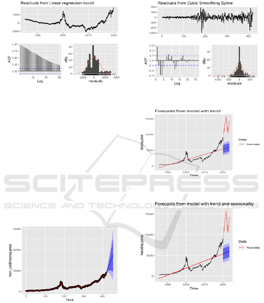
Figure 13: Model with Trend And Seasonality (Picture

credit: Original).

Next, the model with seasonality (Fig 13)

indicating that there is no strong seasonality in the

data, since no seasonality term is significant in this

model. This is also observable from the line plot

given before. Besides, similar results were observed

from the ACF as in the trend model, where the

residuals do not follow a normal distribution and is

non-stationary.

3.6 Using Cubit Spline Fit

The fit in Figure 14 and 15 show that the ACF plot of

the residuals shows some immediate drop-off after 6

lags. Although the Ljung-Box test still gives us a non-

stationary test. Regarding the histogram of the

residual, now it becomes symmetric, but the central

part is much higher than the normal distribution.

Figure 14: Cubic Spline Fit Model (Picture credit:

Original).

Figure 15: Residuals from Cubic Smoothing Spline (Picture

credit: Original).

Figure 16: Forecasting From Model with Trend (Picture

credit: Original).

Figure 17: Forecasting From Model With Trend And

Seasonality (Picture credit: Original).

DAML 2023 - International Conference on Data Analysis and Machine Learning

520

Figure 18: Forecast from Model with Trend And

Seasonality (Picture credit: Original).

Figure 19: Forecast from Model Cubic Spline Regression

(Picture credit: Original).

In comparison of those above models (Figure 16,

17, 18 and 19), the cubic spline method emerges as the

most fitting for capturing the upwards trending of the

Nasdaq index trend. This exhibits superior accuracy

and adaptability of the data. In contrast, models based

on trend and trend-seasonality decomposition did not

perform as well. These simpler models were unable to

capture the model complex fluctuations present in the

Nasdaq index, thereby yielding less accurate forecasts.

4 CONCLUSION

In conclusion, this project aimed to forecast the

Nasdaq index using various time-series methods,

including ARIMA, multiple linear regression, cubic

spline, and trend-seasonality decomposition. The

results indicate a significant correlation between the

Nasdaq index and several economic indicators like

M2 money supply, interest rates, and unemployment

rates. The cubic spline model stood out as the most

accurate and adaptable in capturing the data’s

complex fluctuations. While trend and trend-

seasonality models were found not that accurate. The

ARIMA model, particularly the (0,2,1) configuration,

also showed promise in reflecting real-world upward

trends, despite some initial discrepancies in

stationarity tests. The multiple linear regression

model gave us valuable insights into how different

economic indicators are associated with the Nasdaq

index. Particularly, it fulfilled our initial assumptions

regarding the relevance of these indicators. However,

the trend predicted by the Cubic Spline Fit Model can

be impacted by Covid-19 because the behaviors and

community changed significantly. Overall, the multi-

model approach has allowed people to have an

overview of the Nasdaq index from various angles,

leading to a more nuanced understanding of its

behavior.

REFERENCES

G. W. Schwert, “Stock returns and real activity: A century

of evidence,” The Journal of Finance, 1990, 45(4),

1237-1257.

E. F.Fama and K. R. French, “Common risk factors in the

returns on stocks and bonds,” Journal of Financial

Economics, 1993, 33(1), 3-56.

K. J. Kim, “Financial time series forecasting using support

vector machines,” Neurocomputing, 2003, 55(1-2),

307-319.

N. F. Chen, R. Roll and S. A. Ross, “Economic forces and

the stock market,” The Journal of Business, 1986,

59(3), 383-403.

P. C. Tetlock, “Giving content to investor sentiment: The

role of media in the stock market,” The Journal of

Finance, 2007, 62(3), 1139-1168.

M. Baker and J. Wurgler, “Investor sentiment in the stock

market,” Journal of Economic Perspectives, 2007,

21(2), 129-152.

Nasdaq composite index. (Federal Reserve Economic Data)

FRED. 2023,

https://fred.stlouisfed.org/series/NASDAQCOM.

Last access time : 09.08.2023.

Nadaq Price. Yahoo Finance. 2023,

https://finance.yahoo.com/quote/%5EIXIC/history?p

=%5EIXIC . Last access time : 09.08.2023.

J. J. Choi and Y. Kim, “Technological changes and the

NASDAQ market dynamics,” Technological

Forecasting and Social Change, 2017, 124, 114-124.

S. Richardson and P. Cziraki, “The impact of ESG factors

on tech stock performance: An empirical analysis,”

Journal of Sustainable Finance & Investment, 2019,

9(3), 207-221.

Forecasting Nasdaq Price Index: A Comparative Study of Regression and Time Series Analysis

521