
A Feature-Engineered ARIMA-SARIMA Hybrid Model for Stock
Price Prediction
Jialu Luo
Department of Computer Science and Technology, Nanjing University, Nanjing, China
Keywords: Stock Price Prediction, ARIMA, SARIMA, Feature Engineering.
Abstract: Stock price prediction has long been a challenging yet vital task for investors and financial analysts. This
research presents an innovative approach to enhance the accuracy of stock price predictions through the
integration of the Feature-Engineered Auto-regressive Integrated Moving Average (ARIMA) and the
Seasonal Auto-regressive Integrated Moving Average (SARIMA) hybrid model. The experiment and analysis
reveal the superior predictive performance of the ARIMA-SARIMA hybrid model compared to standalone
ARIMA or SARIMA models. By judiciously integrating seasonal and non-seasonal factors, the hybrid model
mitigates the limitations of individual models in capturing the complex dynamics of stock price movements.
This study opens new avenues for advancing stock price prediction models, offering investors and financial
practitioners a valuable tool for making informed decisions in an increasingly complex and dynamic financial
landscape. The fusion of traditional time-series analysis with feature engineering underscores the potential
for more accurate and reliable stock price forecasts, with implications extending beyond financial markets to
broader domains of time-series forecasting and prediction. Nevertheless, the fluctuations in stock prices are
influenced by multiple factors, many of which lie beyond the predictive capability of existing models. Thus,
while the hybrid model exhibits promising results, the author recognizes that further research is warranted to
incorporate a broader spectrum of influential factors.
1 INTRODUCTION
In the ever-evolving landscape of financial markets,
the ability to predict stock prices accurately holds
immense significance for investors, traders, and
financial institutions. The dynamic nature of stock
markets, influenced by myriad factors, presents a
formidable challenge for price forecasting.
Traditional time-series analysis methods, such as the
ARIMA and the SARIMA models, have long been
employed for this purpose. However, the
effectiveness of these models is often hindered by
their limited capacity to capture the multifaceted
dynamics of stock price movements.
Stock price prediction has been identified as an
important but challenging topic in the research area
of time-series analy-sis (Ren et al 2023). Foreseeing
upcoming stock prices is vital not only for making
investment decisions, but also for charting a
company's expansion, selecting strategic partners,
and appraising the firm's financial position. Relying
solely on analysts' personal experiences and intuition
for analysis and judgment, investors are susceptible
to emotional influences, leading to herd behavior and
irrational decision-making, lead-ing to significant
losses (Deng 2019). As a result, to help analysts and
investors make informed decisions about stock
trading, a scientific and effective research process is
needed. The most commonly used tools are IT
systems implementing technical analysis indicators
(Herwartz 2017). Matenczuk et al and Khang et al
have conducted recent research in this domain.
ARIMA and SARIMA are two commonly used
time series analysis methods employed to capture
trend and seasonality in stock price variations. Both
ARIMA and SARIMA include the components such
as auto-regression, differencing, and moving
averages. Furthermore, SARIMA extends its
capabilities by including seasonal auto-regression,
seasonal differencing, and seasonal moving averages.
Thus, SARIMA excels at capturing the seasonal
fluctuations characteristics of time series data.
Feature engineering is a crucial data processing
step that contributes to enhancing the performance
Luo, J.
A Feature-Engineered ARIMA-SARIMA Hybrid Model for Stock Price Prediction.
DOI: 10.5220/0012814600003885
Paper published under CC license (CC BY-NC-ND 4.0)
In Proceedings of the 1st International Conference on Data Analysis and Machine Learning (DAML 2023), pages 47-53
ISBN: 978-989-758-705-4
Proceedings Copyright © 2024 by SCITEPRESS – Science and Technology Publications, Lda.
47

and accuracy of the predictive models. Its objective is
to extract or create notable features from raw stock
price data, reflecting the underlying and dynamic
trends in the stock market. In stock prediction, apart
from the opening price, closing price, the highest and
the lowest prices, there are many other significant
price features.
The Relative Strength Index (RSI), proposed by J.
Welles Wilder, was initially applied in the futures
market and has been widely used in the stock market
for the past two to three decades (Yun and Rui 2022).
Its principle is to assess the relative strength of buyers
and sellers in the financial market through the rise and
fall of the closing price or index over a certain period,
in order to speculate on the potential changes in stock
prices or future trends.
The moving Averages (MAs) represent the
average stock prices over defined periods.
Incorporating MA features assists the model in
recognizing price trends, price fluctuations, and
providing insights into stock market movements.
Stochastic Oscillator indicators gauge how stock
prices relate to the high-est and lowest prices over a
given period. Introducing it as an external feature
helps the model identify the strength of price trends
and potential turning points.
Effective design and selection of features through
feature engineering are critical components of
successful stock price prediction models.
In this paper, the author introduces a trained
ARIMA-SARIMA hybrid model using data processed
through feature engineering and comprehensively
evaluates this hybrid model.
2 METHOD
2.1 Data Source
The data was obtained from Yahoo Finance, and in
practical usage, the ‘yfinance’ library was used to
fetch the opening price, highest price, lowest price,
and closing price for each day within the period from
January 1, 2012, to September 12, 2023. The author
used 90% of data spanning nearly a decade as the
training set and reserved 10% for the testing set.
Additionally, calculations were made for the 5-day
moving average (MA5), 10-day moving average
(MA10), 20-day moving average (MA20), Relative
Strength Index (RSI), and Stochastic Oscillator (SO)
for each day. Table 1 and Table 2 below present some
examples from the dataset (the table data is for AMZN
stock data).
Table 1: Some Examples in The Dataset.
Date
Open
Close
High
Low
OS
2012-
01-31
9.7000
9.7220
9.7815
9.4850
91.043502
2012-
02-01
8.6905
8.9730
8.9975
8.6000
30.448928
2012-
02-02
8.9825
9.0860
9.0970
8.8400
39.673493
2012-
02-03
9.1415
9.3840
9.3950
9.0945
63.999984
2012-
02-06
9.3140
9.1570
9.3280
9.1460
45.469344
Table 2: Supplements.
Date
MA5
MA10
MA20
RSI
2012-01-
31
9.630800
9.554950
9.251400
66.748001
2012-02-
01
9.547400
9.505050
9.252475
50.469639
2012-02-
02
9.431400
9.441400
9.263000
54.914276
2012-02-
03
9.354500
9.425150
9.288175
57.422250
2012-02-
06
9.264400
9.410400
9.289500
51.620500
2.2 Feature Engineering
Feature engineering in the ARIMA and SARIMA
model primarily focuses on data preprocessing and
transformation to make time series data suitable for
the model. These preprocessing steps enhance the
model's accuracy and robustness, but they typically do
not involve traditional feature extraction or selection
processes because the ARIMA and SARIMA model
does not utilize explicit features. Instead, it relies on
the autocorrelation and moving average properties of
the data for forecasting.
The opening price, closing price, highest price, and
lowest price for each day can be easily retrieved.
Therefore, for the processing of these four features, it
is only necessary to perform some simple data
cleaning by removing data with NaN values and data
that are outliers.
During model training, the author considered not
only the four key features mentioned above but also
introduced external factors such as RSI, MA5, MA10,
MA20, and the stochastic oscillator as influences on
the model.
The MA5, MA10, and MA20 are derived from the
following calculation formula, where MA(P, N)
represents the N-day simple moving average of P. The
formula is:
(1)
During the data preprocessing stage, a 14-day time
window was chosen to calculate the RSI, which was
subsequently used as an external influencing factor for
DAML 2023 - International Conference on Data Analysis and Machine Learning
48

training the model. To calculate RSI, the first step is
to calculate Relative Strength (RS):
(2)
Then, calculate the Relative Strength Index
(RSI):
(3)
The stochastic oscillator, also known as the KD
indicator, is typically described using %K and %D.
The value of %K is cal-culated using the following
formula, where the ‘
’ re-presents the
minimum of the daily lowest stock prices within the
%K time interval, and ‘
’ represents the maxi-
mum of the daily highest stock prices within the %K
time interval:
(4)
Typically, the K value is used to calculate the D
value. It's common to use a 3-day simple moving
average. The formula is:
(5)
During the training of ARIMA and SARIMA
models, the decision to difference the aforementioned
data is determined based on the model parameters.
2.3 Model Selection
The author trained a hybrid stock price prediction
model based on ARIMA and SARIMA using the
processed data. During the training of the hybrid
model, the author employed an automatic parameter
selection function and chose the SARIMA model with
the minimum AIC and the ARIMA model with the
mini-mum BIC, respectively.
2.3.1 ARIMA Model
ARIMA model is a sophisticated and accurate
algorithm proposed by Box and Jenkins for analysing
and forecasting time series data (Shali 2013). In the
ARIMA model, AR stands for autoregressive, I
stands for differencing, and MA stands for moving
average. The AR model captures data with long-term
historical trends and utilizes them for predictions
while the MA model is more suitable for handling
time series data with transient, abrupt changes, or
high noise levels.
The ARIMA model forecasts the future by
exploring autocorrelations between historical data
through methods such as differencing. During model
training, ARIMA relies on three crucial parameters:
p, q, and d, representing the characteristics of its three
constituent parts.
Parameter p represents the characteristic of the
AR component, which determines that the observed
values in the autoregressive model are a linear
combination of the previous p values. Its
mathematical expression with the feature p is as
follows:
(6)
Parameter d represents the characteristic of the I
com-ponent, which represents the order of
differencing.
Parameter q represents the characteristic of the
MA component, which describes the lag values of the
error terms used in the model (i.e., the values from the
previous q periods). Its mathematical expression with
the feature q is as follows:
(7)
As a result, the formula for the ARIMA model can
be expressed as:
(8)
2.3.2 SARIMA Model
The SARIMA and ARIMA models are both
traditional time series forecasting models. The
difference is that SARIMA takes seasonal factors into
account in addition to what ARIMA does. It has three
non-seasonal parameters, namely p, q, and d, and four
seasonal parameters denoted as P, Q, D, and s. The
non-seasonal parameters are defined similarly to the
ARIMA model mentioned earlier.
When defining a SARIMA model, the lag
operator B is introduced. Equation (9) represents the
lag operator B acting at the time
, which is
equivalent to shifting
by one-time step, resulting in
.
(9)
Once defined the lag operator B can be used to
express the differencing operation by a formula:
(10)
Now, define a lag operator polynomial:
(11)
With the above definitions, it is easy to derive
simplified descriptions for ARIMA and SARIMA.
The simplified description of ARIMA is as follows:
(12)
The simplified description of SARIMA (p, d,
q)
is as follows:
(13)
A Feature-Engineered ARIMA-SARIMA Hybrid Model for Stock Price Prediction
49
2.3.3 Parameter Selection Criteria
When determining the parameters of the ARIMA-
SARIMA hybrid model, suitable parameters can be
found by observing the ACF, PACF, and EACF plots,
as well as by computing the values of AIC and BIC.
In this article, the parameters are determined using the
AIC and BIC evaluation criteria.
The AIC and BIC serve distinct purposes. While
the AIC aims to approximate models to match real-
world situations, the BIC strives to identify the best-
fit model. BIC tends to favour relatively simpler
models and imposes a strong penalty on model
complexity. On the other hand, AIC emphasizes
model fit, which is often beneficial for time series
data with clear seasonality and trends, making it more
suitable for SARIMA models. By choosing a
combination of ARIMA (with the lowest BIC) and
SARIMA (with the lowest AIC), it is possible to
better adapt to different types of time series data.
When training the ARIMA-SARIMA hybrid
model, the main objective is to minimize the values
of AIC and BIC by selecting different parameters.
Smaller values of AIC and BIC indicate higher model
fitness, which correspondingly leads to improved
prediction accuracy. The ARIMA model can handle
relatively stationary data more effectively, while the
SARIMA model excels at capturing seasonality and
trends. The author used the ‘auto_arima’ function
from the ‘pmdarima’ library for automatic parameter
selection.
2.4 Evaluation Criteria
2.4.1 Residual Analysis
Residuals are the differences between model
predictions and actual observed values. Conducting
residual analysis helps assess whether the model can
capture the underlying structure in the data and
whether the residuals meet model assumptions, such
as independence and constant variance.
(14)
2.4.2 Rolling Forecast
Apply the model to the first-time point in the test set
to make the initial prediction. Then, add the observed
value to the training set and retrain the model. Repeat
this process until all time points in the test set have
been predicted. Calculate the prediction error for each
time point and assess the model's performance.
2.4.3 Cross-Validation
Divide the time series data into k folds, and for each
fold, use it as the test set while the remaining folds
serve as the training set. Fit an ARIMA-SARIMA
model on each fold and make predictions on the test
set. Calculate the prediction error for each fold.
3 RESULT
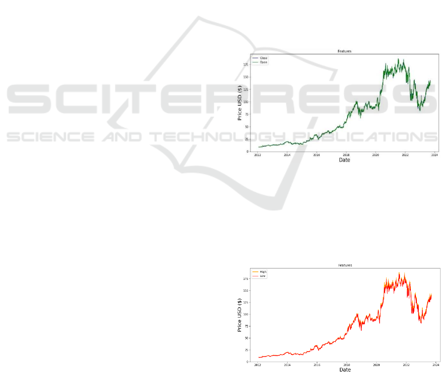
3.1 Feature Visualization
The following charts illustrate some of the key features
of Amazon (AMZN) stock over the past decade. In this
context, the closing price was chosen as the primary
feature, with RSI, SO, MA5, MA10, and MA20 being
considered as external influencing factors. The
opening and closing prices shown in Figure 1 were
extracted from data obtained from Yahoo Finance. A
simple data cleaning process was performed, removing
entries with NaN values and outliers.
Figure 1: The daily closing price and opening prices of
Amazon stock. (Picture credit: Original).
The daily highest and lowest prices shown in Fig.
2 were also extracted from data obtained from Yahoo
Finance. A simple data cleaning process was also
performed, removing entries with NaN values and
outliers.
Figure 2: The daily highest price and lowest prices of
Amazon stock. (Picture credit: Original).
DAML 2023 - International Conference on Data Analysis and Machine Learning
50
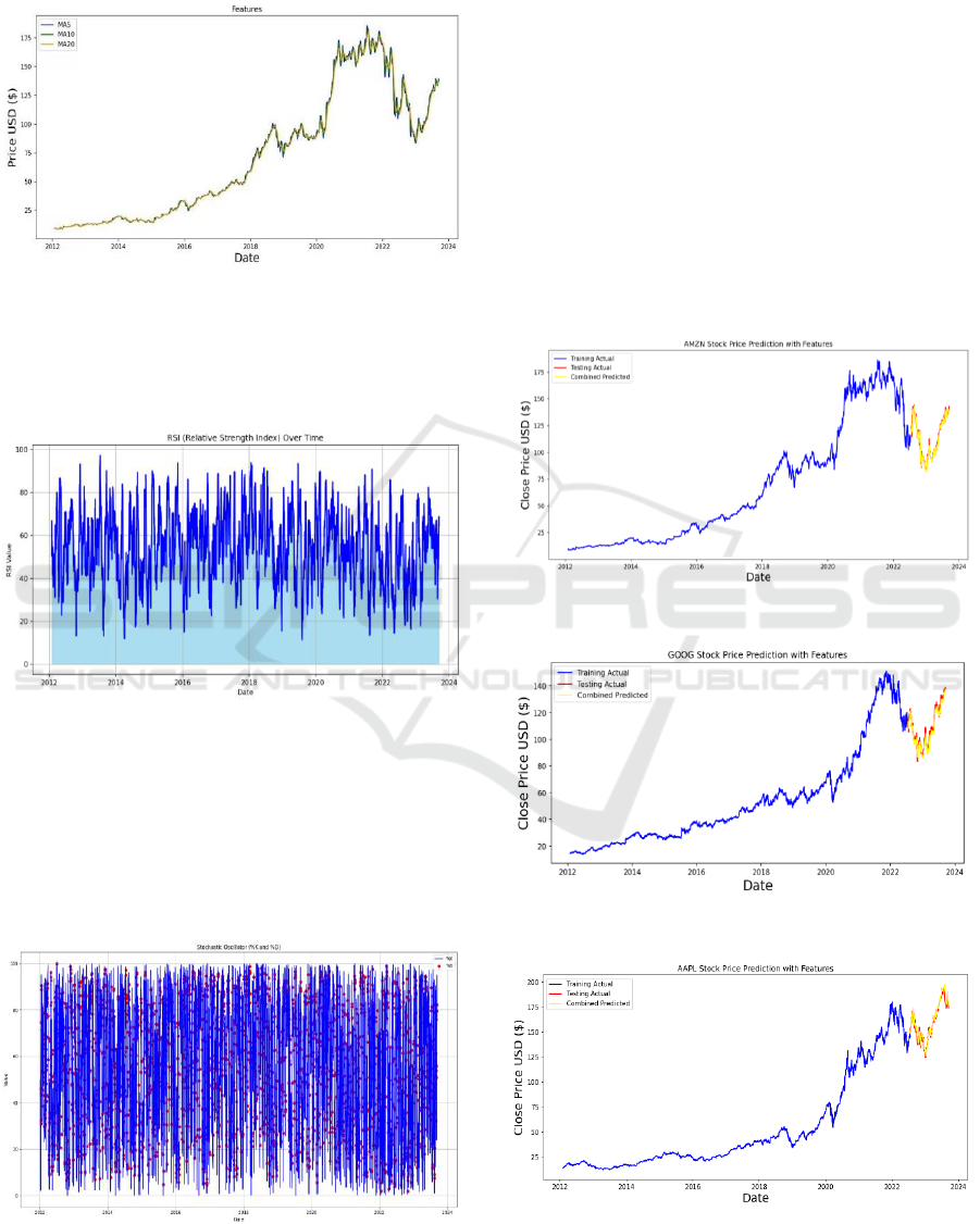
The data for these three features shown in Fig. 3
are calculated using the formula mentioned earlier in
the paper.
Figure 3: The daily moving average for the last five days,
ten days, and twenty days (MA5, MA10, MA20) of
Amazon stock. (Picture credit: Original).
The RSI shown in Fig. 4 below is calculated with
a time window of 14 periods.
Figure 4: The daily RSI of Amazon stock. (Picture credit:
Original).
In the Stochastic Oscillator visualization chart
(Fig. 5), the Main (%K) is represented as the blue solid
line, while the Signal (%D) is represented as the red
dots. The %K period is the period used in the
calculation of the oscillation indicator, with a default
value of 5.
Figure 5: The daily Stochastic Oscillator of Amazon stock.
(Picture credit: Original).
3.2 Predict Results
From Fig. 6, Fig. 7, and Fig. 8, it can be observed that
the ARIMA-SARIMA hybrid model achieves high
accuracy in predictions and does so within a very short
execution time. The results shown in the figure below
are based on a dataset obtained from the ‘yfinance’
library, which includes the daily opening, closing,
highest, and lowest stock prices of the respective
company over the past decade. After completing the
data preprocessing mentioned in this article, the data
was used for training and testing the hybrid model.
And 90% of the data was used as the training set, while
the remaining 10% was used as the test set. The red
curve represents the actual data of the test set, while
the yellow curve represents the results predicted by the
model.
Figure 6: AMZN Stock Price Prediction. (Original).
Figure 7: GOOG Stock Price Prediction. (Original).
Figure 8: AAPL Stock Price Prediction. (Original).
A Feature-Engineered ARIMA-SARIMA Hybrid Model for Stock Price Prediction
51
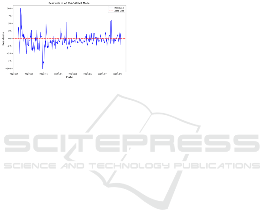
3.3 Evaluation
Fig. 9 displays the residual plot of the hybrid model,
demonstrating properties such as zero mean and
randomness. Fig. 9 depicts the residuals obtained
from the predictions for AMZN stock.
Figure 9: Residuals of ARIMA-SARIMA Model. (Picture
credit: Original).
The Mean Squared Error (MSE) of the hybrid
model obtained through rolling forecasting and cross-
validation is consistently less than 2.21. The author
conducted numerous model training for the AMZN
stock and calculated the average MSE from each
iteration. The average MSE of the hybrid model is
2.1914293478806233.
Under otherwise identical conditions, the average
MSE for predictions using a single ARIMA model i
s 2.579234434378756, and for a single SARIMA mo
del, it is 2.3328237024728707.
4 DISCUSSION
Numerous models have been developed in the
financial literature to predict return and volatility, but
the ARIMA model is the most widely used, which was
published by Arnerić & Poklepović in 2016 (Arnerić
et al 2014). Nevertheless, the ARIMA-SARIMA
hybrid model outperforms single ARIMA or
SARIMA models in terms of predictive capability.
This indicates that in stock prediction, there is a
combination of seasonal and non-seasonal factors.
However, the author reckons that hybridizing ARIMA
and SARIMA models might be a somewhat
adventurous endeavor. The hybrid model in this paper
precisely complements the seasonal factors that
ARIMA lacks with SARIMA and compensates for the
non-seasonal factors that SARIMA overlooks with
ARIMA. Through the assumed research and empirical
simulation analysis of the aforementioned quantitative
environment, the hybrid model proposed in the paper
yielded relatively favorable results in specific trading
contexts. This suggests that employing tools for
quantitative trading offers certain advantages.
Quantitative trading, due to its reliance on the rapid
and robust computational capabilities of computers,
holds an absolute advantage in market breadth
analysis (Li and Xia 2023). However, the factors
influencing stock price trends in the actual market are
intricate and diverse. Therefore, if various political
and economic factors affecting the stock market are
considered alongside technical indicators as input
variables, better results may be obtained (Agrawal et
al 2013).
5 CONCLUSION
The stock price prediction model has been effectively
deployed using the aforementioned techniques, with
feature engineering emerging as a crucial step in
enhancing prediction accuracy for this regression
problem. In an effort to enhance stock price prediction
accuracy, this study aspires to introduce a fresh
perspective. Nonetheless, given the multitude of
factors influencing stock prices, the current model's
performance may not be entirely satisfactory. To
enhance the model's effec-tiveness, future research
should consider incorporating a wider array of factors.
REFERENCES
S. Ren, X. Wang, X. Zhou, Y. Zhou, “A novel hybrid model
for stock price forecasting integrating Encoder Forest
and Informer,” Expert Systems with Applications,
Volume 234, 2023, 121080, ISSN 0957-4174,
https://doi.org/10.1016/j.eswa.2023.121080.
F.X. Deng, “Application of LSTM Neural Network in Stoc
k Price Trend Prediction,” Master's thesis, Guangdong
University of Foreign Studies, 2019, https://kns.cnki.n
et/kcms2/article/abstract?v=InnWydrwIfKm2Z35Pntd
CsfBawT604FUNihTlaJLVNqnhwfaWN2kRbqki1Rd
MbUheTK2Jlwt62CDDuzq1y4XMGZfX6rsdojNBX4
W5a9KbSVOrrjLI6JZT74wL9yytntgCzw4WYEVzXo
=&uniplatform=NZKPT&language=CHS.
H. Herwartz, “Stock return prediction under GARCH — An
empirical assessment,” International Journal of
Forecasting, vol. 33, pp. 569-580, 2017.
W. Budiharto, “Data science approach to stock prices
forecasting in Indonesia during Covid-19 using Long
Short-Term Memory (LSTM),” Journal of Big Data,
vol. 8, 2021.
J. Pomponi, S. Scardapane, and A. Uncini, “Structured
Ensembles: an Approach to Reduce the Memory
Footprint of Ensemble Methods,” Neural Networks,
vol. 144, pp. 407-418, 2021.
Y. Yun and Y. Rui, “Application Validity Test of RSI Indi
cator in Bond Trading Decision,” Modern Business, no
DAML 2023 - International Conference on Data Analysis and Machine Learning
52

36, pp. 123-126, 2022, https://doi.org/10.14097/j.cnki.
5392/2022.36.023.
Shali, “Research on Regional Electricity Consumption
Forecasting Method Based on ARIMA Model and
Regression Analysis,” Master's thesis, Nanjing
University of Science and Technology, 2013.
J. Arnerić, T. Poklepović, and Z. Aljinović, “GARCH based
artificial neural networks in forecasting conditional
variance of stock returns,” Croatian Operational
Research Review, vol. 5, pp. 329-343, 2014.
X. Li and H. Xia, “Research on Stock Price Regression
Prediction Based on Machine Learning Algorithms,”
Science and Technology Information, no. 14, pp. 227-
231, 2023.
J. Agrawal, V.S. Chourasia, and A.K. Mittra, “State-of-the-
Art in Stock Prediction Techniques,” International
Journal of Advanced Research in Electrical, Electronics
and Instrumentation Energy, vol. 2, pp. 1360-1366,
2013.
A Feature-Engineered ARIMA-SARIMA Hybrid Model for Stock Price Prediction
53
