Classification of GALAXY, QSO, and STAR Based on KNN and PCA

Zhichen Lin

School of Computing and Artificial Intelligence, Southwest Jiaotong University, Chengdu, China

Keywords: Celestial Bodies Classification, KNN, PCA, Standard Scaler.

Abstract: As science and technology have advanced over the past few years, numerous astronomical measurement

technique projects—like the Sloan Digital Sky Survey (SDSS)—have been built and implemented. Many

astronomical data has been collected, including the characteristic data of galaxies, stars, and other celestial

bodies. The classification of a large amount of astronomical data requires an efficient algorithm. In this paper,

a galaxy (GALAXY), star (STAR), Quasi-Stellar Object (QSO) classification model was constructed using

machine learning techniques and the Sloan Digital Sky Survey - DR18 dataset. Different algorithms, including

K-Nearest Neighbors (KNN) and Principal Component Analysis (PCA), were used to build this model. The

obtained model in this paper exhibits good performance indicators, with accuracy rates of 96%, 98%, 96%,

and 98%, respectively. To decrease the dimensionality of the data, the author employed PCA and discovered

that certain information in the data was irrelevant to the classification. Discarding these irrelevant features

can speed up the training process. The importance of classifying celestial bodies based on astronomical data

is evident, as it helps people better understand the composition and evolution of the universe and has

significant implications for predicting and explaining astronomical phenomena. However, the same type of

celestial body may have significant differences in certain features and practical scenarios, so a more extensive

and higher-quality training set is needed to train better-performing models. These models can help people

classify celestial bodies more quickly and accurately

1 INTRODUCTION

Under the ongoing advancements in technological and

scientific fields, many astronomical surveying

techniques projects have been constructed and used,

such as the Sloan Digital Sky Survey (SDSS) (York et

al 2000). A vast amount of astronomical data has been

collected. The importance of classifying celestial

bodies based on these astronomical data is evident, as

it helps people better understand the composition and

evolution of the universe and holds significant

significance for predicting and explaining

astronomical phenomena. However, celestial body

classification is also filled with challenges. The same

type of celestial body may vary significantly in certain

characteristics, and the vast amount of

multidimensional astronomical data and observational

results place considerable demands on the algorithms

and computational capabilities used to process and

analyze this data. Therefore, it is necessary to

determine the most suitable machine-learning

techniques for classifying celestial bodies. For

example, studies based on stacking ensemble studying

for celestial body classification have established basic

classifier models using algorithms like Random

Forests and Support Vector Machines (Luqman et al

2022). In their paper, using Multi-label K-Nearest

Neighbors (ML-KNN), a KNN algorithm-based

approach, Zhang and Zhou experiment with multi-

class studying issues. And ML-KNN performs better

than several well-known multi-class learning

techniques (Zhang and Zhou 2007). The performance

suggests that KNN has certain advantages in handling

large multi-label problems. The paper by Logan and

Fotopoulou employed PCA for data preprocessing in

the categorization of three celestial bodies. The PCA

performed in this paper reduced the input attributes to

approximately 2-5 dimensions (Logan and

Fotopoulou 2020).

PCA, or principal component analysis, is a method

for extracting the most essential information from a

data table and simplify the description of the dataset

(Abdi and Williams 2010). It is a powerful data

analysis tool that can help detect patterns, reduce data

dimensions, and identify outliers. One of its

fundamental applications is reducing the number of

Lin, Z.

Classiﬁcation of GALAXY, QSO, and STAR Based on KNN and PCA.

DOI: 10.5220/0012814900003885

Paper published under CC license (CC BY-NC-ND 4.0)

In Proceedings of the 1st International Conference on Data Analysis and Machine Learning (DAML 2023), pages 54-60

ISBN: 978-989-758-705-4

features in a dataset to alleviate the computational

burden of machine learning algorithms.

The Standard Scaler feature scaling technique

normalizes each feature by narrowing the variance to

one and subtracting its mean. which effectively

prevents the significant differences in magnitudes

among various features from causing certain features

to dominate the model training, thereby preventing a

decrease in the accuracy of the model training.

However, there are also some drawbacks to the

Standard Scaler, including its vulnerability to values

that deviate from the normal range and preference for

normally distributed data (Ferreira et al 2019).

In this paper, the authors employ various methods,

including KNN, PCA-KNN, and Standard Scaler, to

classify GALAXY, QSO, and STAR, three types of

celestial bodies.

2 METHOD

2.1

Dataset

The dataset is called Sloan Digital Sky Survey - DR18.

It comprises 100,000 observations from the Data

Release (DR) 18 of the Sloan Digital Sky Survey

(SDSS). Each observation data consists of 42 different

features. Based on these 42 feature values, the

observation data is classified into a GALAXY, a

STAR, or a QSO. Among them, 52343 rows are

GALAXY, 37232 are STAR, and 10425 are QSO.

Table 1 shows some examples of the dataset.

Table 1: Some examples in the dataset.

class

features

redshift expAB_u petroFlux_z field

GALAXY

0.04169106 0.04169106 207.0273 462

STAR 0.000814368 0.04169106 4.824737 467

GALAXY 0.1130687 0.7016655 278.0211 467

STAR 8.72E-05 0.9998176 134.6233 467

STAR 1.81E-05 0.9997948 388.3203 467

STAR -8.72E-05 0.8620063 185.476 467

2.2 Plitting the Dataset

In this research, the author randomly divided the

dataset into 80% training and 20% testing sets.

Stratified sampling was conducted based on the class

proportions to ensure that the proportions of each class

in the training and testing sets were similar.

2.3

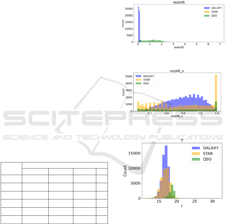
Dataset Visualization

Each distinct feature is different in GALAXY, STAR,

and QSO. The following pictures show some

visualized results. 0, 2, and 3 illustrate three different

features among these three celestial bodies.

Figure 1: Different characteristics of the 'redshift' in

GALAXY, STAR, QSO (Picture credit: Original).

Figure 2: Different characteristics of the 'expAB_u' in

GALAXY, STAR, QSO (Picture credit: Original).

Figure 3: Different characteristics of the 'r' in GALAXY,

STAR, QSO (Picture credit: Original).

The author used box plots to visualize the

distribution of data. As shown in Figure 4, if the upper

and lower whiskers are relatively long, it indicates a

significant variation in the data beyond the upper and

lower quartiles, suggesting a larger overall variance

and standard deviation, which can significantly impact

model training.

Classiﬁcation of GALAXY, QSO, and STAR Based on KNN and PCA

Figure 4: Box plot of 6 features (Picture credit: Original).

Each different feature is unique for the three types of

celestial bodies. There are a total of 42 features.

However, not all features strongly correlate with the

classes of celestial bodies, so the author has created a

correlation heatmap of all the features. After being

selected by the author, the correlation between the 14

features and the categories of celestial bodies is shown

in Figure 5. These 14 features exhibit a strong

correlation with the classes of celestial bodies.

Figure 5:Part of the Correlation Heatmap (Picture credit:

Original).

Meanwhile, the author also calculated the

correlation between each class and all the features.

Meanwhile, the author also calculated the correlation

between each class and all the features.

A significant positive correlation (n >= 0.7) has

been found for one feature with "class_GALAXY";

six features have a moderate positive correlation (n <

0.7 && n >= 0.5); six feature have a weak positive

correlation (n < 0.5 && n > 0); and 29 features have a

negative or zero correlation (n <= 0).

One feature with "class_QSO" has a strong

positive correlation (n >= 0.7); one feature has a

moderately positive correlation (n < 0.7 && n >= 0.5);

four features have a weak positive correlation (n < 0.5

&& n > 0); and thirty-six features have a 0 or negative

correlation (n <= 0).

The data indicates that there are 34 features with 0

or negative correlation (n <=0), 3 features with

moderately positive correlation (n < 0.7 && n >= 0.5),

5 features with weakly positive correlation (n < 0.5

&& n > 0), and no features with substantially positive

correlation (n>=0.7) with "class_STAR".

2.4 Algorithm

The author first uses Standard Scaler to normalize the

data in this project. Then, the author uses PCA to

decrease the data dimensionality. Then, the author

trains a KNN model based on these reduced-

dimensional datasets for classifying GALXY, STAR,

and QSO.

Standard Scaler:Normalization of data. One

feature scaling technique is Standard Scaler. By

deducting the mean from each feature and scaling the

variance to one, it can be made normal. It can scale

features with different scales to the same range,

avoiding the excessive influence of certain features on

the model, which is crucial for the KNN model in this

experiment, as the distance calculation of KNN will

be dominated by features with larger scales if there are

significant differences in feature scales. Scaling the

dataset will lead to more accurate results than not

scaling it. The box plot illustrates that the dataset for

this experiment has different value ranges for different

features. Therefore, normalization is required for this

dataset (Raju et al 2020). For each feature, including

S observed value, calculate its mean 𝑋



, where each

observation in the feature is 𝑋



, and use equation 1 to

determine the normalized 𝑋





















(1)

where

𝜎





∑















(2)

PCA: Dimensionality reduction of data. One

popular method for reducing dimensionality is

Principal Component Analysis, or PCA. It is applied

to convert high-dimensional data into a space with

fewer dimensions. It reduces dimensionality by

identifying the primary directions of variance in the

original data and projecting the data onto these

directions. Principal Component Analysis first

calculates the covariance matrix to describe the linear

relationship between each feature, given data with s

number of samples, where the covariance matrix is

obtained by:

∑







∑

𝑥



−𝑥̅





𝑥



−𝑥̅



(3)

Where

𝑥̅ 





∑

𝑥







(4)

DAML 2023 - International Conference on Data Analysis and Machine Learning

PCA performs eigenvalue decomposition on the

covariance matrix to obtain their corresponding

eigenvectors. Then, it selects the top N principal

components based on the magnitude of the

eigenvalues, where N is the desired dimensionality

after dimension reduction and defined by the author.

After calculating the quantities of different PCs, sort

the retained data information and select the top 25 PCs

to train the KNN model.

KNN: Prediction. K-Nearest Neighbors represents

one of the machine learning techniques used for

classification as well as regression. It is used to

classify three types of celestial bodies. The KNN

algorithm stores each feature data in the training set.

In this research, for one sample data in the test set, the

KNN algorithm calculates the k points with the

smallest Euclidean distance to this sample point. It

classifies this sample data into the category of the

nearest neighbors. The accuracy generally changes

with the variation of the k value. Because K-NN

merely stores the training dataset at first and only uses

it to figure out how to categorize or predict new

datasets as necessary, it is sometimes referred to as a

lazy learning algorithm (Bansal et al 2022). In their

paper, Niu and Lu et al0 noted that various distance

metrics are crucial and significantly impact nearest-

neighbor-based algorithms (Niu et al 2013). In this

paper, the author uses Euclidean distance. KNN

Euclidean distance formula:



∑

(𝑥



−𝑦



)







(5)

2.5 Evaluation Criteria

Confusion matrix: The confusion matrix counts the

number of samples in the incorrect category and the

right group. The forecast outcomes are displayed in

the confusion matrix. It displays conflicted forecast

outcomes. It can not only assist in mistake detection

but also error type display. At the same time, the

confusion matrix makes it simple to compute other

high-level classification indicators.

Accuracy: Percentage of accurate predictions. It is

one of the most commonly used metrics in multi-class

classification, and its formula considers the sum of

correctly predicted examples as the numerator and the

sum of the confusion matrix's total entries as the

denominator (Grandini et al 2020). It represents

accurately predicted test samples’ percentage out of all

the test samples in this study.

𝐴𝑐𝑐𝑢𝑟𝑎𝑐𝑦 =





(6)

Macro Average Precision (MAP): Average of each

category's precision, which is the proportion of

accurate predictions among the anticipated positive

instances. In the STAR devision, the denominator is

the number of correctly identified examples in the

STAR category divided by the number of examples

identified as the STAR category in non-STAR

examples. The numerator is the number of correctly

identified examples in the STAR category in the true

situation.

𝑀𝑎𝑐𝑟𝑜𝐴𝑣𝑒𝑟𝑎𝑔𝑒𝑃𝑟𝑒𝑐𝑖𝑠𝑖𝑜𝑛 =





∑

















(7)

Macro Average Recall (MAR): It is the average

value of the recall rate for each category. In this

research, The recall rate represents the percentage of

samples that the model correctly predicts as belonging

to a certain class out of all the actual samples

belonging to that class.

𝑀𝑎𝑐𝑟𝑜𝐴𝑣𝑒𝑟𝑎𝑔𝑒𝑅𝑒𝑐𝑎𝑙𝑙 =





∑

















(8)

Macro F1-Score: Macro F1-Score is the name

given to the harmonic mean of Precision and Recall.

Because MAR or MAP cannot be used independently

to assess a model, the Macro F1-score balances the

two indicators and makes them compatible. The

algorithms that perform well across all categories

exhibit a high Macro F1-score, while the algorithms

with inaccurate predictions demonstrate a low Macro

F1-score (Grandini et al 2020).

𝑀𝑎𝑐𝑟𝑜𝐹1 −𝑠𝑐𝑜𝑟𝑒=

 ∗ 









(9)

3 RESULT

3.1 Data Dimensionality Reduction

The author compared the explained variance,

accuracy, and training time in the experiment when

using from 1 to 25 principal components

(PCA(n_components=i)) and KNN. The metrics can

be seen in 0, 0, and 0.

The explained variance, in 0, increases with the

number of PCs. However, the rate of its increase

gradually slows down. After the number of PCs

reaches 23, there is no significant increase, indicating

that the maximum amount of information has been

retained when the number of PCs reaches 23.

In Fig. 7, the more PCs there are, the higher the

accuracy rate. But after there are five PCs, the pace of

increase slows down. The accuracy increases slightly

when the number of PCs is between 5 and 20.

However, the accuracy no longer improves when the

number of PCs exceeds 20.

Classiﬁcation of GALAXY, QSO, and STAR Based on KNN and PCA

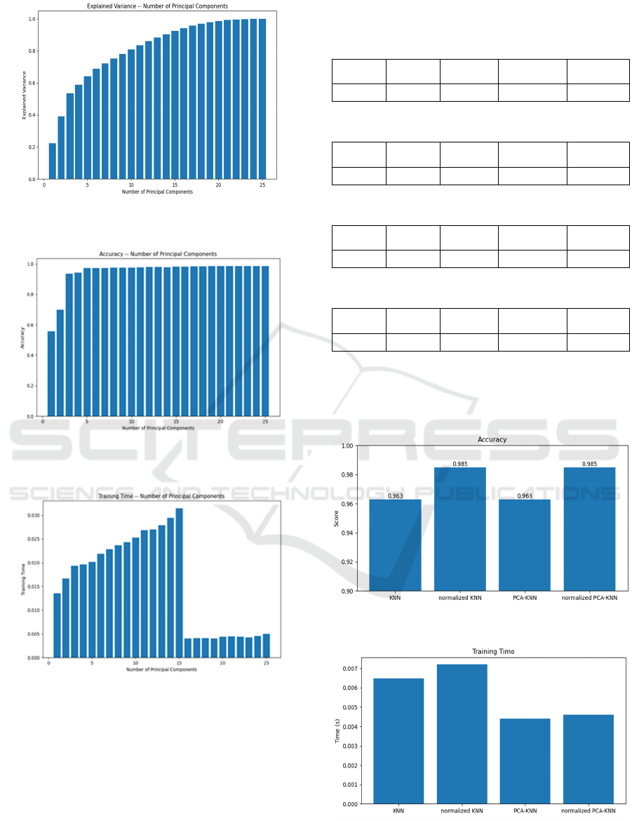
Figure 6: Explained Variance and Number of PCs (Picture

credit: Original).

Figure 7: Accuracy and Number of PCs (Picture credit:

Original).

Figure 8: Training Time and Number of PCs (Picture credit:

Original).

0 demonstrates a continuous increase in training

time between 1PCs and 15 PCs. However, at 16 PCs,

the training time suddenly decreases and remains

stable between 16 PCs and 23 PCs.

When PC is set to 23, it retains the main variance,

achieves relatively high accuracy, and significantly

reduces training time. Therefore, the author decided

to use 23 PCs for the subsequent analysis.

3.2 Predict Result

Table 2: Predict results of KNN.

MAP MAR

Macro

F1-score

Accuracy

training

time

0.96 0.94 0.95 0.96 0.0065s

Table 3: Predict results of normalized KNN.

MAP MAR

Macro

F1-score

Accuracy

training

time

0.99 0.97 0.98 0.98 0.0072s

Table 4: Predict results of PCA-KNN.

MAP MAR

Macro

F1-score

Accuracy

training

time

0.96 0.94 0.95 0.96 0.0044s

Table 5: Predict results of normalized PCA-KNN

MAP MAR

Macro

F1-score

Accuracy

training

time

0.98 0.97 0.98 0.98 0.0046s

From 0, 0, 0, 0, it can be observed that KNN,

normalized KNN, PCA-KNN, and normalized PCA-

KNN all exhibit high accuracy, high MAP, and high

MAR while requiring relatively short training time.

Figure 9: Accuracy of different models (Original).

Figure 10: Training Time of different models (Original).

DAML 2023 - International Conference on Data Analysis and Machine Learning

In Figure 9 and 10, the KNN model trained on the

data set normalized by Standard Scaler shows

improved accuracy compared to the original KNN

algorithm. However, the training time has also

increased accordingly. Therefore, when evaluating

the advantages and disadvantages of different

algorithms, it is crucial to consider the specific usage

scenario and the clients' customized requirements.

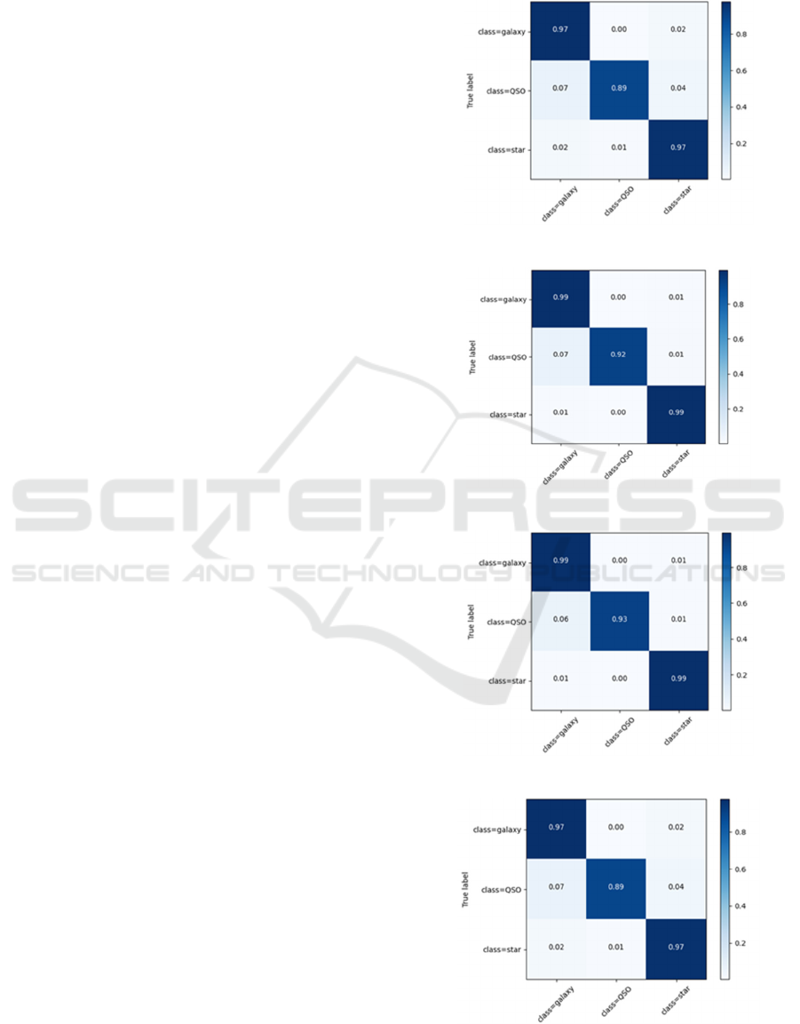
3.3 Evaluation

The confusion matrix is used to count the amount of

specimens that are classified correctly or incorrectly.

The y label represents the true label, while the x label

represents the predicted label by the model. For

example, the number in the square corresponding to

the first galaxy class on the x-labels and the second

QSO class on the y-labels is the proportion of the

model predicting the QSO class as galaxy class.

These confusion matrices, displayed in 0, 12, 13,

and 14, demonstrate excellent accuracy. However, it

can be observed from the figures that the model tends

to classify QSO as GALAXY in the test set. The

author believes this is the model's primary source of

error.

DISCUSSION

The training time of the model is short, allowing for

multiple training sessions in a short period. In addition,

the precision, recall, and accuracy are all very high.

The charts in the results show that the accuracy of the

normalized KNN model reaches 98.5%, which is an

improvement compared to KNN's 96.3%. Furthermore,

all performance metrics have improved, indicating that

Standard Scaler significantly enhances the reliability of

the data. Compared to KNN, PCA-KNN has the same

performance metrics and reduces data dimensionality,

resulting in a noticeable reduction in training time. This

suggests that some feature information is irrelevant

when classifying these three types of celestial bodies.

Normalized PCA-KNN incorporates data

normalization and dimensionality reduction steps,

achieving the same performance metrics as normalized

KNN while only taking 2/3 of the training time.

Moreover, it outperforms PCA-KNN in

performance metrics while maintaining a similar

training time. Normalized PCA-KNN trains faster

than normalized KNN, significantly reducing training

time while improving accuracy, Macro Average

Precision, and other metrics. In the future, the

normalized PCA-KNN model can be used in many

other regression and classification tasks involving

many features, some of which may be irrelevant.

Figure 11: KNN (Picture credit: Original).

Figure 12: normalized KNN (Picture credit: Original).

Figure 13: PCA-KNN (Picture credit: Original).

Figure 14: normalized PCA-KNN (Picture credit: Original).

Classiﬁcation of GALAXY, QSO, and STAR Based on KNN and PCA

5 CONCLUSION

The GALAXY, STAR, and QSO classification model

has been successfully implemented using four

different techniques. Among them, normalized

PCA+KNN is more suitable for this small-scale

classification problem in terms of performance,

computation time, and cost. This research aims to

provide new insights into celestial object

classification to help people classify celestial objects

more practically. However, due to the limited dataset,

the model's current performance may only partially

be satisfactory. The author must add more extensive

and more diverse datasets to future research to

improve the model's effectiveness.

REFERENCES

D. G. York et al., "The sloan digital sky survey: Technical

summary," The Astronomical Journal, vol. 120, no. 3,

p. 1579, 2000.

A. Luqman, Z. Qi, Q. Zhang, and W. Liu, "Stellar

Classification by Machine Learning," SHS Web of

Conferences, vol. 144, 2022, doi:

10.1051/shsconf/202214403006.

M.-L. Zhang and Z.-H. Zhou, "ML-KNN: A lazy learning

approach to multi-label learning," Pattern Recognition,

vol. 40, no. 7, pp. 2038-2048, 2007, doi:

10.1016/j.patcog.2006.12.019.

C. Logan and S. Fotopoulou, "Unsupervised star, galaxy,

QSO classification-Application of HDBSCAN,"

Astronomy & Astrophysics, vol. 633, p. A154, 2020.

H. Abdi and L. J. Williams, "Principal component

analysis," Wiley interdisciplinary reviews:

computational statistics, vol. 2, no. 4, pp. 433-459,

2010.

P. Ferreira, D. C. Le, and N. Zincir-Heywood, "Exploring

feature normalization and temporal information for

machine learning based insider threat detection," in

2019 15th International Conference on Network and

Service Management (CNSM), 2019: IEEE, pp. 1-7.

V. G. Raju, K. P. Lakshmi, V. M. Jain, A. Kalidindi, and V.

Padma, "Study the influence of

normalization/transformation process on the accuracy

of supervised classification," in 2020 Third

International Conference on Smart Systems and

Inventive Technology (ICSSIT), 2020: IEEE, pp. 729-

735.

M. Bansal, A. Goyal, and A. Choudhary, "A comparative

analysis of K-Nearest Neighbor, Genetic, Support

Vector Machine, Decision Tree, and Long Short Term

Memory algorithms in machine learning," Decision

Analytics Journal, vol. 3, 2022, doi:

10.1016/j.dajour.2022.100071.

J. Niu, B. Lu, L. Cheng, Y. Gu, and L. Shu, "Ziloc: Energy

efficient wifi fingerprint-based localization with low-

power radio," in 2013 IEEE Wireless Communications

and Networking Conference (WCNC), 2013: IEEE, pp.

4558-4563.

M. Grandini, E. Bagli, and G. Visani, "Metrics for multi-

class classification: an overview," arXiv preprint

arXiv:2008.05756, 2020.

DAML 2023 - International Conference on Data Analysis and Machine Learning