Classification of Fruits Based on CNN, SVM and PCA

Qianming Huang

School of Information Engineering, China University of Geosciences Beijing, Beijing, China

Keywords: Fruits Classification, CNN, SVM, PCA.

Abstract: In today's time, fruits are a daily necessity for human beings and people use a lot of fruits daily. To meet the

demand for fruits, the total global production of fruits in 2019 was about 740 million tonnes, according to the

Food and Agriculture Organisation of the United Nations (FAO). The timely handling of these fruits is

undoubtedly an important issue, especially since fruits are characterized by a short shelf life. Therefore, the

use of various types of machines to process fruits has become a research direction in today's world, and this

includes the recognition and classification of fruit images by machines. This paper is based on a machine

learning approach to construct models from fruit image datasets. Two models are used in this paper which are

the SVM model with PCA and, the CNN model. Both models obtained good classification accuracy

respectively, 90% for the SVM model and 97% for the CNN model. But the SVM model training time took

only 2.73s whereas the CNN model training took 120.09s. Therefore, to pursue a certain level of efficiency,

SVM+PCA was chosen as the model for fruit classification in a good situation where the lights are bright and

the fruits are not covered.

1 INTRODUCTION

Fruit is really common in People's Daily life. Every

adult over the age of 18 needs to consume more than

114.8 grams of fruit every day (Liu et al 2022). In

today's digital age, advances in machine learning and

image processing have provided a unique opportunity

to solve a variety of practical problems. Among them,

the fruit classification problem is a challenging

research area. There are so many kinds of fruits in

different forms that distinguishing them is a relatively

easy task for humans, but it is difficult to translate into

a problem that can be recognized and distinguished

by computers. Because the current fruit classification

is mainly carried out manually, a quarter of the fruits

in China cannot be processed in time and rot every

year (Wang 2018), which undoubtedly makes a huge

waste. Therefore, it is of great research value and

practical significance to use machine learning

algorithms to solve fruit classification problems.

Image classification has emerged as a prominent

research area due to the advancements in computer

vision technology. People try to use K-Nearest

Neighbor (KNN), Support Vector Machines (SVM),

and many other traditional machine-learning

algorithms to classify images. For example, Liu et al.

introduced a technique for segmenting MRI images.

The SVM is trained to classify the medical images

(Liu et al 2011). C. Arun Priya also used a support

vector machine to classify plants by using five

principal variables as input vectors. The five principal

variables are obtained from 12 leaf features (Priya et

al 2012). People have also tried to use deep learning

algorithms, and most of the algorithms for solving

image classification problems are based on

Convolutional Neural Network (CNN). Q. Li

suggested using CNN to identify lung image patches

associated with interstitial lung disease (ILD) (Li et al

2014). Besides, to classify fruits, S.lu designed a six-

layer CNN comprising convolution layers, pooling

layers, and fully connected layers. (Lu et al 2018).

Deep learning algorithms outperform traditional ML

in image classification accuracy. However,

traditional machine learning algorithms have more

advantages in the time required for model training. So

far, there is no research to show which machine-

learning algorithm is better for fruit classification.

A commonly used machine learning algorithm for

classification tasks is Support Vector Machine (SVM).

It separates the samples of different classes as much as

possible in the sample space by finding an optimal

hyperplane. SVM has powerful nonlinear

classification ability and can deal with complex

nonlinear relationships by mapping samples to high-

Huang, Q.

Classiﬁcation of Fruits Based on CNN, SVM and PCA.

DOI: 10.5220/0012815000003885

Paper published under CC license (CC BY-NC-ND 4.0)

In Proceedings of the 1st International Conference on Data Analysis and Machine Learning (DAML 2023), pages 457-465

ISBN: 978-989-758-705-4

457

dimensional space through kernel function. Using the

Radial Basis Function as a kernel function can make

SVM have better performance in classification

accuracy (Hussain et al 2011). SVM also has good

generalization ability and is robust to noisy data

(Cortes and Vapnik 1995). While SVM performs well

on a small dataset, its training time significantly

increases with a large dataset. However, the increase in

classification accuracy is relatively small. To achieve

efficient training of an SVM model, it is necessary to

reduce the dimensionality of the features.

Principal Component Analysis (PCA) is a widely

used technique for dimensionality reduction By

identifying principal components that capture

maximum data variance, PCA simplifies dataset

complexity and enhances computational efficiency.

Because of the above properties of PCA, a primary

application of PCA is to reduce the computational

workload of a machine learning algorithm by

reducing the number of features in the dataset.

A widely used deep learning model in computer

vision tasks is the Convolutional Neural Network

(CNN). It can effectively process and extract features

in an image by using components such as

convolutional layers. CNN uses the convolution

operation to slide on the input image, and learns the

weight of the convolution kernel (filter) to realize the

extraction of local features in the image (Simonyan

and Zisserman 2014), and has the ability of

translation invariance (Bruna and Mallat 2013). By

stacking multiple convolutional and pooling layers,

CNN can learn more abstract and high-level feature

representations layer by layer. Finally, through the

fully connected layer and Softmax activation

function, CNN can map the extracted features to

different categories to realize image classification.

Compared with the traditional Neural Network (NN),

CNN has advantages in processing image data due to

its local perception and parameter-sharing

characteristics (LeCun et al 1998).

In this paper, SVM+PCA and CNN are used to

classify fruits. According to the data produced by the

two methods, the comprehensive performance of the

two methods for fruit classification problems is

obtained, to evaluate the two methods, and finally

obtain an objective conclusion.

2 METHOD

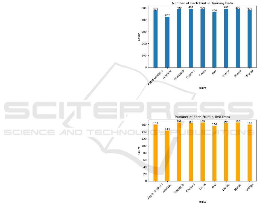
2.1 Dataset

The dataset is called Fruit 360 (Kaggel). This dataset

includes fruits and vegetables of various kinds. The

dataset contains a total of 90,483 images. There are

67,692 pictures in the training set, with each image

containing either a fruit or a vegetable. The test set

consists of 22,688 images, where each image contains

either a fruit or a vegetable. A total of 131 classes are

included, encompassing various types of fruits and

vegetables. All the images dealt with flood fill

algorithm which can make the background of the

images to be uniform. Some examples in the dataset

are shown in Figure 1 and Figure 2.

Figure 1: Several fruits in the training dataset (Picture

credit: Original).

Figure 2: Several fruits in the test dataset (Picture credit:

Original).

2.2 Data Visualization

Nine different fruits were selected from the dataset

for demonstration. These fruits have similar

appearances, which poses a challenge for

classification algorithms. If these nine similar fruits

can be well classified, then the classification

algorithm can still perform better for a greater variety

of fruits. These nine fruits are shown in Figure 3.

DAML 2023 - International Conference on Data Analysis and Machine Learning

458

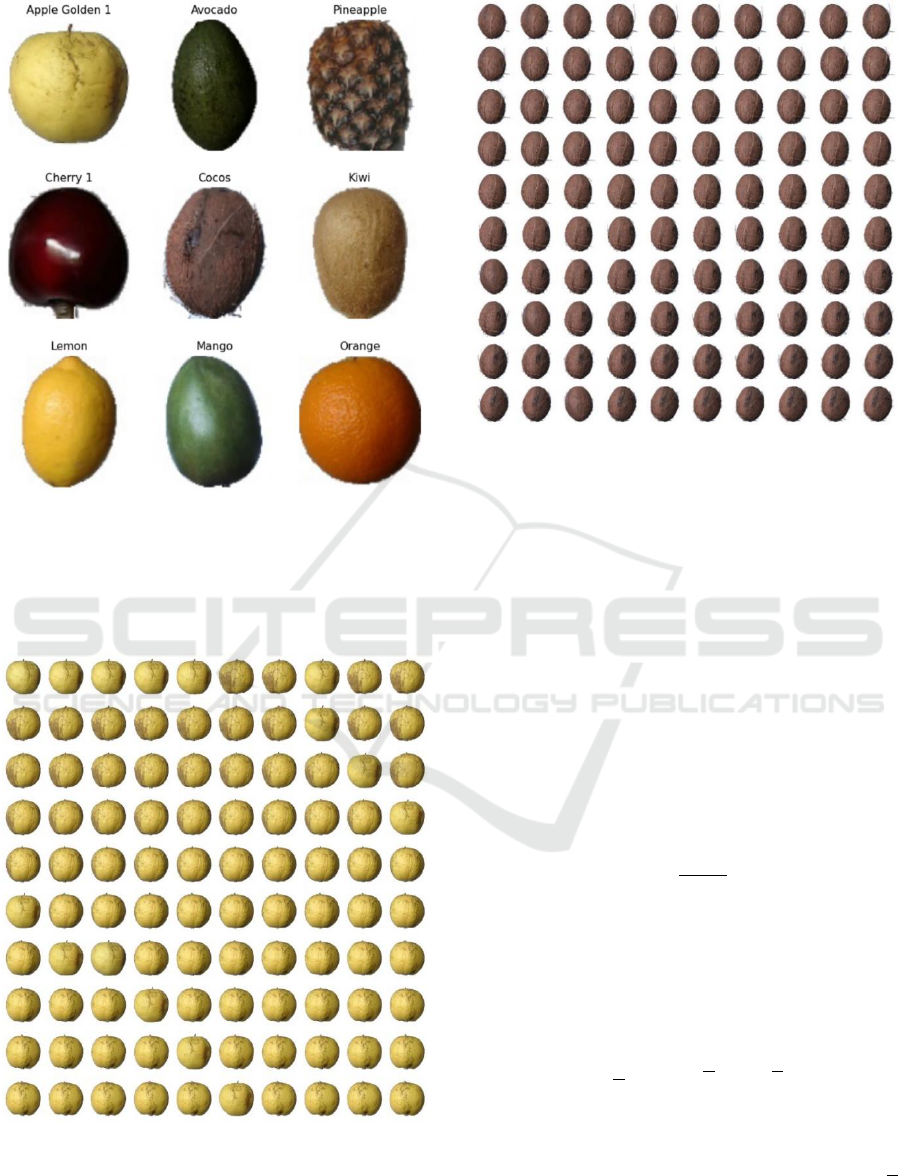
Figure 3: Nine similar fruits (Picture credit: Original).

Each fruit was also photographed from different

angles and directions. Figure 4 and Figure 5 show

several pictures of two kinds of fruits in the dataset.

Figure 4: Some pictures in the dataset of Apple Golden 1

(Picture credit: Original).

Figure 5: Some pictures in the dataset of Cocos (Picture

credit: Original).

2.3 Algorithm

2.3.1 PCA

PCA is a linear transformation method that projects

the original high-dimensional data into a new low-

dimensional space by finding the direction of the

maximum variance in the data to achieve

dimensionality reduction and feature extraction.

When PCA is performed, the data first needs to be

standardized. For every sample, the eigenvalue is

subtracted from the mean of the entire dataset and

divided by the variance to ensure that each feature has

a unit variance. The standardized data can be

expressed as:

 

 









In the given equation,  represents the raw data,

 denotes the mean value of the entire data set, and 

represents the data variance.

The next step is to calculate the covariance matrix.

The covariance matrix can be obtained by the

following formula:

Σ 





































In the given equation,  symbolizes the total

number of samples present in the dataset, 



represents the standardized sample eigenvalue, and 

denotes the mean value of the complete dataset.

Classiﬁcation of Fruits Based on CNN, SVM and PCA

459

The covariance matrix reflects the relationship

between different features in the original data.

Then, eigenvectors and eigenvalues may be

produced via eigenvalue decomposition of the

covariance matrix. The primary component directions

are represented by the eigenvectors, and the

accompanying eigenvalues denote the significance of

the corresponding eigenvectors.

The process of getting eigenvectors and

eigenvalues is shown in the following.

Let the covariance matrix be Σ, the eigenvectors

be , and the eigenvalues be . The expression for

eigenvalue decomposition is as follows.

Σ  







The covariance matrix can be subjected to

eigenvalue decomposition to provide a collection of

eigenvectors 











and associated eigenvalues













, where  is the feature vector's

dimension.

To select the most important principal

components, the corresponding eigenvalues are

sorted from largest to smallest :





 



   









The eigenvectors with the largest eigenvalues are

chosen as principal components to represent the most

important information in the original data.

A new set of orthogonal eigenvectors can be

obtained through these steps, which are called

principal components. Principal components project

the original data into a new feature space, where each

principal component represents a part of the salient

information in the original data.

2.3.2 SVM

Finding the best hyperplane in the high-dimensional

feature space to employ in separating the various fruit

sample groups as much as feasible is the basic idea

behind SVM. SVM finds a hyperplane defined by

support vectors to maximize classification

performance and generalization. ‘rbf’ is used as a

kernel function.

2.3.3 K-Fold

In this fruit classification study, K-fold was employed

to assess the ability of the machine learning

algorithm.

The dataset is divided into K folds, with K-fold

performing training on    folds, validation on 1

fold, repeating this process K times, and finally

calculating the average results for performance

evaluation.

Using K-fold cross-validation offers several

benefits in this fruit classification research. Firstly, it

maximizes the utilization of the limited dataset by

training and validating the model on different subsets.

This helps to ensure that the model works well to

unseen fruits. Additionally, K-fold cross-validation

helps to mitigate any potential bias or variance issues

that may arise from using a single validation set.

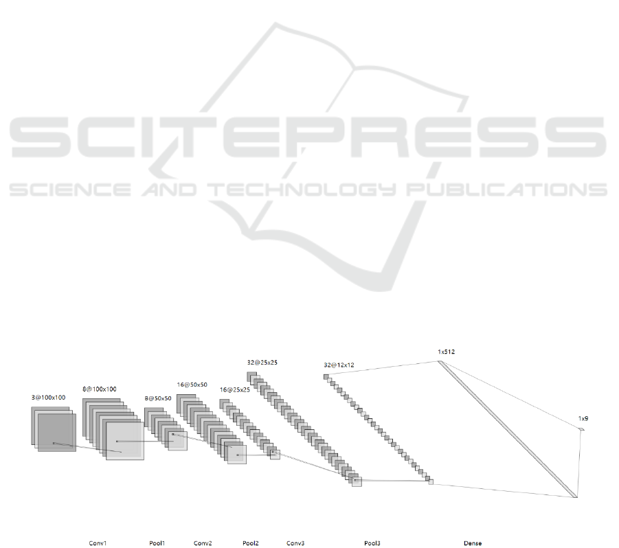
2.3.4 CNN

As shown in Figure 6, there are several layers in the

CNN model. Dropout is also included in each layer to

mitigate the overfitting problem and improve the

generalization ability of the model. In addition, data

enhancement was performed on the dataset before

training.

2.4 Activation Function

The ReLU function is a commonly used nonlinear

activation function that helps neural network models

to better fit nonlinear relationships by retaining the

positive part and clipping the negative part. It has the

Figure 6: Network architecture (Picture credit: Original).

DAML 2023 - International Conference on Data Analysis and Machine Learning

460

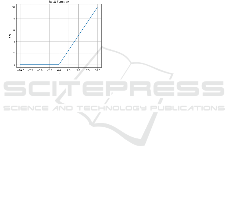
advantages of sparsity, fast convergence, and avoiding

gradient vanishing.

The mathematical formula for the ReLU function

can be expressed as:









 





 





In the given function, x represents the input value,

while f(x) represents the output value generated by the

ReLU function. The expression states that if the input

x is positive, the output will be equal to x; otherwise,

the output will be 0. The image of the ReLU function

is shown in Figure 7.

Figure 7: ReLU Function (Picture credit: Original).

2.5 Convolutional Layer

Convolutional layer is an important component in

deep learning neural networks. It extracts features

from the input image by using convolutional

operations and generates a corresponding feature map

as output. For a three-dimensional input image (e.g.,

an RGB image), the convolutional layer performs

convolutional operations on the width, height, and

channel dimensions of the image.

The mathematical formula can be expressed as:









 







  





















Where 







denotes the values of the elements

in the output feature map of the convolutional layer,





 



denotes the values of the pixels at a

particular location in the input image, and 







denotes the value of the weights of the convolutional

kernel.

Convolutional operations are performed by sliding

a learnable convolution kernel over the input image

multiplying it element by element with the pixel values

at the corresponding positions on the image, and

summing these products to obtain the convolution

result. Multiple convolution kernels can be used to

extract different features or to increase the depth of the

network.

The benefit of a convolutional layer is that it

preserves the local features and positional information

of the input image and the model doesn’t have to learn

too many parameters. What’s more, the layer makes

the model more translation invariant by sharing

weights, i.e., the same features can be detected at

different locations.

2.6 Pooling Layer

The pooling layer usually is used to decrease the

complexity of the model, reduce the number of

parameters, and improve the robustness and

generalization of the model. Pooling operations are

performed on various regions of the feature map and

the values within each region are pooled to obtain an

output value.

Max Pooling is chosen for modeling because Max

Pooling extracts the most significant features in the

regions while reducing the size of the feature map.

2.7 Evaluation

2.7.1 Confusion Matrix

Confusion matrices are an important tool for

evaluating model performance in classification

problems. It provides detailed information about the

relationship between the model predictions and the

actual labels.

The confusion matrix is comprised of four main

components: True Positive (TP), True Negative (TN),

False Positive (FP), and False Negative (FN). They

describe the case of different prediction outcomes.

Confusion matrix gives detailed performance

evaluation information for the model. By examining

the confusion matrix, one can compute additional

metrics like macro-P to evaluate the model’s ability.

2.7.2 Accuracy

Accuracy is calculated by dividing the number of

correctly classified samples (True Positives and True

Negatives) by the total number of samples, and it

measures the overall correctness of the model's

predictions:

 

 

    







2.7.3 macro-R

Recall is a measure of how many of all the samples in

Classiﬁcation of Fruits Based on CNN, SVM and PCA

461

which the model is actually a positive case are

correctly predicted as positive cases. Calculating the

macro-R value gives an overall idea of the model's

recall for each category.

For each category , calculate the recall 



for that

category:

























Calculate the average of the recall for all

categories as macro-R:

 



















 





Where 











denote the recall of each

category respectively and n denotes the total number

of categories.

2.7.4 macro-P

The value of macro-P gives an idea of the average

accuracy of the model on each category, and each

category is given the same weight.

For each category , calculate the precision 



for

that category:

























The average precision for all categories is macro-P:

 















 



 





Where 











denote the precision of each

category respectively and n denotes the total number

of categories.

2.7.5 macro-F1

Macro-F1 serves as a comprehensive performance

metric that reflects the model's ability to balance

prediction accuracy and checking completeness in a

multi-class classification task and provides a fair

assessment of performance across classes. The macro-

F1 is calculated using the following formula:

 





 



 







RESULT

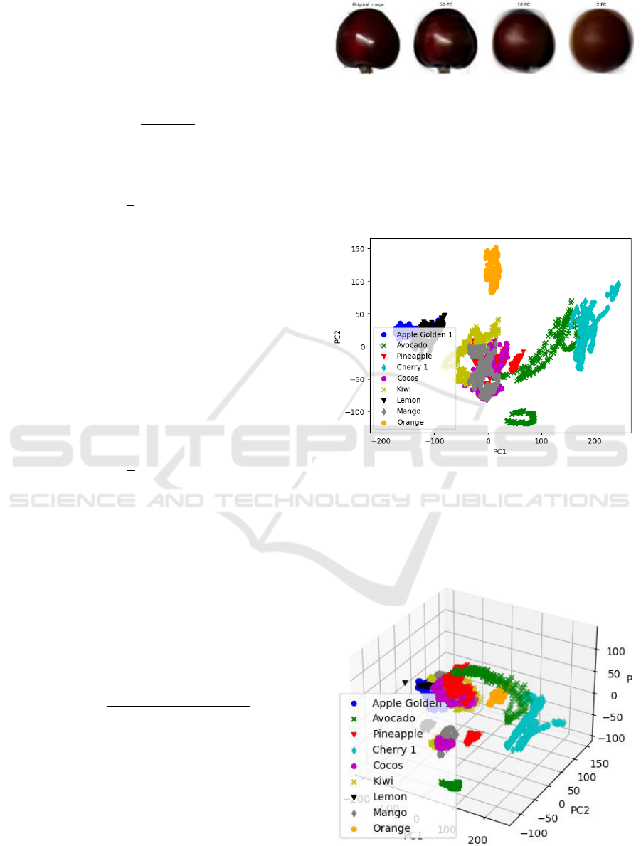
2.8 The Result of PCA

A series of principal components can be obtained by

the formula of PCA. As the number of selected

principal components decreases, the image will

become increasingly blurred and will have fewer and

fewer features. As shown in Figure 8, when pc is equal

to 2, it is almost impossible to see that this is a cherry.

Figure 8: Images of cherry corresponding to different

numbers of principal components (Picture credit: Original).

As Figure 9 shows when a principal component is

equal to two, it's hard to separate different kinds of

fruit. Mango, pineapple, and coconut are mixed

together. There is a partial overlap between Golden

Apple and Lemon. Avocado and Cherry also partially

overlap. Only Orange is well-separated.

Figure 9: Dataset with two principal components (Picture

credit: Original).

When the principal component is equal to 3. There

are more fruits in the dataset that can be separated.

Orange and Avocado in Figure 10 can be well

separated.

Figure 10: Dataset with three principal components (Picture

credit: Original).

DAML 2023 - International Conference on Data Analysis and Machine Learning

462

2.9 Classification Result

2.9.1 SVM+PCA

Two kinds of experiments were carried out for the

SVM algorithm, and RBF was used as the kernel in

both experiments. The first experiment is SVM+PCA,

and the second experiment is SVM+PCA+K-Fold.

The results of the experiment are as follows.

Table 1: Predict results of SVM+PCA.

PCA

macro

-P

trainin

g time

macro

-F1

Accurac

macro

-R

0.60

2.06s

0.56

0.55

0.56

0.70

1.46s

0.65

0.64

0.65

1.78s

0.23

0.24

0.25

0.79

2.69s

0.15

0.11

0.12

0.90

3.68s

0.03

0.11

0.90

5.81s

0.02

0.11

0.90

7.21s

0.02

0.11

0.90

8.26s

0.02

0.11

According to Table 1, when PCA is equal to 2,

Accuracy is the highest and macro-F1 is also the

highest. With the increase of PCA, all the other

variables decrease except macro-P, and the training

time also becomes longer. When PCA is 8 or higher,

all values tend to stabilize. But the change in training

time is obvious.

Table 2: Predict results of SVM+PCA+K-FOLD, when

PCA is equal to 2.

K-

Fold

macro-

training

time

macro-

Accuracy

macro-

0.47

1.41s

0.36

0.37

0.74

1.48s

0.73

0.72

0.73

0.79

1.50s

0.79

0.78

0.79

0.80

1.50s

0.80

0.83

1.54s

0.83

According to Table 2, with the increase of K-Fold,

all values increased. When the K-Fold is 10 or higher,

most values remain stable without significant

improvement. But the increase in training time was

larger.

Table 3: Predict results of SVM+PCA+K-FOLD, when

PCA is equal to 5.

K-

Fold

macro-

training

time

macro-

Accuracy

macro-

0.80

2.77s

0.09

0.13

0.14

0.85

2.72s

0.72

0.68

0.86

2.68s

0.79

0.77

0.90

2.74s

0.85

0.83

0.84

0.90

2.73s

0.91

0.90

According to Table 3, most observed values are

gradually improved, and at the same time, the training

time remains relatively stable.

Table 4: Predict results of SVM+PCA+K-FOLD, when

PCA is equal to 8.

K-

Fold

macro-

training

time

macro-

Accuracy

macro-

0.8

3.70s

0.08

0.13

0.91

3.62s

0.67

0.61

0.92

3.68s

0.76

0.70

0.71

0.93

3.68s

0.80

0.72

0.77

0.94

3.67s

0.88

0.86

According to Table 4, most observed values are

gradually improved, but the training time is longer. In

particular, when K-Fold is increased from 10 to 15,

there is a huge improvement in Accuracy.

Considering Table 2, Table 3, and Table 4, it can

be seen that when PCA is equal to 5 and K-Fold is

equal to 15, most values are the best, and the training

time is acceptable.

2.9.2 CNN

Table 5: Predict results of CNN.

macro-P

training

time

macro-

Accuracy

macro-R

0.97

120.09s

0.97

In Tabel 5, most values are excellent, reaching 0.97.

But the training time of 120s is a little longer.

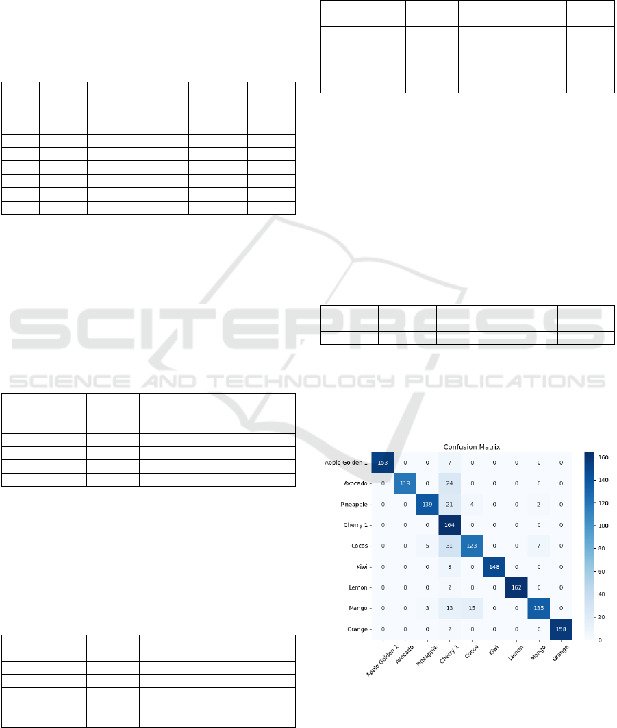
2.10 Confusion Matrix

Figure 11: Confusion matrix of SVM+PCA (Picture credit:

Original).

Classiﬁcation of Fruits Based on CNN, SVM and PCA

463

As can be seen from Figure 11, SVM+PCA performs

better for the classification of three types of fruits,

namely Cherry 1, Lemon, and Orange, and worst for

Avocado. Many fruits are incorrectly recognized as

Cherry 1 and Cocos; however, this problem does not

have a significant impact on real-world applications

because, in real-world scenarios, Cherry 1 has a

significant size difference from other fruits, which

means that it can be easily distinguished.

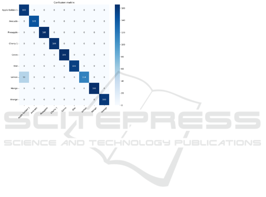
Figure 12: Confusion matrix of CNN (Picture credit:

Original).

As can be seen from Figure 12, the CNN model

performs very well for the fruit classification problem,

and can accurately classify fruits. The fruits in the

validation set are correctly distinguished except for

Lemon. The small part of Lemon is classified as Apple

Golden 1. This may be because Apple Golden 1 is too

similar to Lemon in some perspectives, which leads to

the model's inability to classify them accurately.

3 DISCUSSION

Both the SVM+PCA model and the CNN model

obtained relatively good results for the same dataset.

The CNN model, because of its effective capture of

local spatial features, parameter sharing, and weight

sharing properties, thus obtained up to 97% Accuracy

and possessed a more accurate classification

performance than the SVM model on the test set. The

SVM model does not have as high a classification

accuracy as the CNN model, but it also has an

Accuracy of 90%, which is a good result.

In addition, thanks to the SVM model having

fewer parameters, relying only on support vectors for

training, and using convex optimization methods

during training, the SVM+PCA model used less time

in the face of a large dataset, only 2.73s, which is

1/44th of the time used by the CNN model. Therefore,

SVM possesses higher efficiency. If the dataset is

further expanded, the advantage of the SVM model in

training time will be more obvious.

In the future, when faced with better-use

environments (e.g., supermarkets, in which there are

bright environments and fruits are not obscured),

SVM models can help people quickly classify and

recognize fruit items. In poorer environments (e.g.,

field picking environments, where fruits may be

obscured by leaves), the CNN model, with its higher

classification accuracy, can better help people classify

and recognize fruits, and even assist machine picking.

This study still has some shortcomings. The first is

that the dataset is not big enough or rich enough. This

leads to a smaller range of applicability of the trained

model. If pictures of fruits in different scenarios are

introduced, such as apples in shadows or cherries

obscured by leaves, then a better model can be

obtained. In addition, there is a shortage of hardware

equipment. In the future, better hardware equipment

can be used. This can not only cope with larger

datasets but also build more complex models.

4 CONCLUSION

The SVM model and CNN model are used for the fruit

classification problem. The comprehensive

performance of the SVM model and CNN model for

the current dataset is obtained separately through

extensive experiments to know the best performance

of these two models. For the problem of fruit

classification in a good situation, the SVM model is

more appropriate because although its classification

accuracy is slightly worse than the CNN model, the

time consumed for training is much better than the

CNN, and the accuracy of the SVM+PCA is also

acceptable.

In the future, this model can be used in robots to

help people sort fruits. In addition, this technology can

also be used in cell phones and other smart terminal

devices to help people identify unknown fruits.

REFERENCES

C. Y. Liu, L. M. Wang, X. X. Gao, Z. J. Huang, X. Zhang,

Z. P. Zhao, …, and M. Zhang (2022). Study on

DAML 2023 - International Conference on Data Analysis and Machine Learning

464

vegetable and fruit intake status among Chinese adults

in 2018. Chinese Journal of Chronic Diseases

Prevention and Control, (08), 561-566.

doi:10.16386/j.cjpccd.issn.1004-6194.2022.08.001.

S. T. Wang (2018). Research and Design of Embedded Fruit

Automatic Classification System [Master’s thesis,

Huazhong Normal University].

Y. T. Liu, H. X. Zhang, and P. H. Li (2011). Research on

SVM-based MRI image segmentation. The Journal of

China Universities of Posts and Telecommunications,

18, 129-132.

C. A. Priya, T. Balasaravanan, and A. S. Thanamani (2012,

March). An efficient leaf recognition algorithm for plant

classification using support vector machine. In

International conference on pattern recognition,

informatics and medical engineering (PRIME-2012)

(pp. 428-432). IEEE.

Q. Li, W. Cai, X. Wang, Y. Zhou, D. D. Feng, and M. Chen

(2014, December). Medical image classification with

convolutional neural network. In 2014 13th

international conference on control automation robotics

& vision (ICARCV) (pp. 844-848). IEEE.

S. Lu, Z. Lu, S. Aok, and L. Graham (2018, November).

Fruit classification based on six layer convolutional

neural network. In 2018 IEEE 23rd International

Conference on Digital Signal Processing (DSP) (pp. 1-

5). IEEE.

M. Hussain, S. K. Wajid, A. Elzaart, and M. Berbar (2011,

August). A comparison of SVM kernel functions for

breast cancer detection. In 2011 eighth international

conference computer graphics, imaging and

visualization (pp. 145-150). IEEE.

C. Cortes, and V. Vapnik (1995). Support-vector networks.

Machine learning, 20, 273-297.

K. Simonyan, and A. Zisserman (2014). Very deep

convolutional networks for large-scale image

recognition. arXiv preprint arXiv:1409.1556.

J. Bruna, and S. Mallat (2013). Invariant scattering

convolution networks. IEEE transactions on pattern

analysis and machine intelligence, 35(8), 1872-1886.

Y. LeCun, L. Bottou, Y. Bengio, and P. Haffner (1998).

Gradient-based learning applied to document

recognition. Proceedings of the IEEE, 86(11), 2278-

2324.

Kaggel. (n.d.). Fruits 360 Dataset. Retrieved from

https://www.kaggle.com/datasets/moltean/fruits

Classiﬁcation of Fruits Based on CNN, SVM and PCA

465