Classification of Fruits Based on Convolutional Neural Networks

Shaoyang Zhang

College of Computer and Information, Hohai University, Nanjing, China

Keywords: Fruits Classification, Image Recognition, Convolutional Neural Network.

Abstract: Large-scale agricultural electrification and automation are inseparable from the assistance of computer

science. However, traditional automation equipment is mainly used in relatively single operations that do not

require identification or rely on manual classification and identification. An improvement to this condition is

to provide electronic devices with higher-accuracy automatic classification capabilities. Image recognition

technology is an essential part of this improvement. Convolutional neural network is a commonly used and

effective technology to achieve image recognition. Therefore, this paper takes fruit as an example and uses

some models based on convolutional networks for recognition and classification. The paper uses some

relatively accurate methods and achieves high accuracy in recognizing images containing a single fruit.

However, one of the problems of this paper is that the paper does not cover the processing and recognition of

complex images. The model in this article may have some flaws in complex real-life situations. Improvements

to this problem include obtaining more complex data sets and model modifications.

1 INTRODUCTION

Since its birth, computers have undertaken the

mission of simplifying calculations for humans. The

delivery of computer vision shows that computers

have the ability to replace humans in making

judgments to a certain extent. Computer vision

attempts to use machine programs to achieve a

human-like or even greater ability to recognize

images. In recent years, this technology has continued

to develop, and computer vision no longer stays in the

laboratory but instead participates in solving complex

real-life problems (Islam 2022). Traditional

agricultural technology benefits from combining

deep learning and computer vision and is gradually

moving toward automation (Dhanya et al 2022). As

an essential part of agriculture, the vegetable and fruit

industry has broad application prospects for computer

vision. The fruit classification mentioned in this

article is a practice of this theme.

Image processing uses deep learning technology to

achieve breakthroughs in automation with the help of

computers (Chen et al 2023). Each module of deep

learning is not complex; they abstract a small part of

the input in the form of numbers and introduce non-

linear functions in the process. The entire network will

gradually combine these modules, and their abstraction

capabilities will gradually increase and begin to show

obvious discrimination capabilities. Finally, the

functions represented by neural networks will be very

complex (LeCun et al 2015). It's very feasible to use

deep learning methods to process fruit images.

Deep learning has great potential in many fields.

Convolutional neural networks are good at handling

some vision-related problems (Yu, Jia and Xu 2017).

Convolutional neural networks (CNN) have

experienced decades of development, and multiple

classic models have been proposed. LeNet-5 is a

classic structure that was put into practical use in

1998. The emergence of convolutional neural

networks began with the LeNet-5 network proposed

by LeCun (Lecun et al 1998). VGG-16 is a famous

CNN model showing that the depth to 16-19 weight

layers can be significantly improved over existing

technical configurations (Simonyan and Zisserman

2014). Many breakthroughs in various fields related

to digital data recognition, such as voice recognition

and image processing have been achieved by

convolutional neural networks (Albawi et al 2017).

Convolutional neural network is highly effective and

most commonly used in diverse computer vision

applications (Guo et al 2016).

One way to improve the accuracy of convolutional

neural networks and make them more effective is to

scale up the convolutional network (Tan and Le 2019).

However, simple expansion is not always effective and

Zhang, S.

Classiﬁcation of Fruits Based on Convolutional Neural Networks.

DOI: 10.5220/0012815100003885

Paper published under CC license (CC BY-NC-ND 4.0)

In Proceedings of the 1st International Conference on Data Analysis and Machine Learning (DAML 2023), pages 361-366

ISBN: 978-989-758-705-4

361

sometimes encounters problems. ResNet uses residual

networks to enhance the capability of neural networks

while scaling up the number of layers and achieving

great success (He et al 2016).

Based on the actual situation, this paper attempts

to improve the capabilities of models and explores the

possibility of using them in fruit classification. In this

paper, the author uses the methods of convolution

neural networks and residual networks to recognize

fruits and achieve higher recognition performance.

2 METHOD

2.1 Dataset

The dataset used in this article is called Fruits 360

(hereafter abbreviated as fruits) (Oltean 2020).

Fulfilling with images of fruits and vegetables, fruits

has an amount of images, which is 90,483. The

training size is 67,692 images, while the test size is

22688. An overview of the data distribution can be

roughly shown in Fig. 1. below.

Figure 1: Number of images for some types of fruit in fruits

(Picture credit: Original).

2.2 Data Preprocessing

Like other non-intuitive data, image information can

be stored in an array or matrix for processing. The

higher the pixels of the image, the larger the matrix

used to represent the image. In fruits, the training and

testing datasets provide a standardized size with 100

pixels in both height and width. In this case, the

standardized input of the models mentioned later in

this article is [100, 100, 3], as the color is divided into

three dimensions. At the same time, this article uses

the linear function to map the data set so that the pixel

value of the image is altered from an integer value

between 0 and 255 to a float value between 0 and 1.

2.3 Deep Learning Algorithm

2.3.1 Convolutional Neural Network

The convolutional neuron network is suitable for

processing and recognizing image information.

Convolutional neural networks can directly process

data without too much preprocessing, greatly

simplifying the data preprocessing steps. At the same

time, it reduces the amount of calculations and

memory usage and improves computing efficiency.

Convolutional neural networks usually include

convolutional, pooling, and fully connected layers to

achieve data processing and analysis.

2.3.2 Convolutional Layers

The convolution layer achieves convolution

processes on the data. In this step, the convolution

kernel will perform operations similar to weighted

superposition with the set size one by one according

to the step size, and the results will be summarized

into a matrix. The core of the convolution operation

is to continuously identify certain features of the

image by designing specific convolution kernels and

ultimately achieve image recognition. Theoretically,

each convolution kernel can recognize part of the

information of the input image.

2.3.3 Pooling Layers

The pooling operation can downsample the input to

reduce the number of parameters. The pooling layer

will divide the matrix according to the pooling kernel

size and step size into new matrices with these small

matrices of the same size as the pooling kernel as

elements and replace each component of these

matrices with the maximum value in the small matrix

or the average weight of each element of the small

matrix. The kernel in this step in this article generally

takes a size of (2, 2) and a step size of 2. In this way,

the length and width of the input after pooling are

reduced to half of the original size.

2.3.4 Fully Connected layers

Each neuron in the fully connected layer needs to

receive all the information from the previous group of

neurons. Before that, the data needs to be flattened

after several convolutions and pooling. This

connection process can be understood as combining

DAML 2023 - International Conference on Data Analysis and Machine Learning

362

the features learned in the previous convolution steps

to achieve the recognition of the whole image.

2.3.5 Residual Block

The residual network can establish direct data

provision between neurons by skip connections,

making it less prone to the phenomenon of vanishing

gradients than conventional convolutional neural

networks (He et al 2016). With this feature, the

residual network has more layers as a matter of course.

2.3.6 Models

In this paper, the author used three neural network

models. Model 1., model 2., and model 3. are used on

behalf of these models here and later. Model 1.

Contains two convolutional layers. Each convolutional

layer is connected to a pooling layer to halve the

abscissa and ordinate the output of the convolutional

layer. Finally, two fully connected layers are used for

connection. Model 2. includes seven convolutional

layers, three pooling layers, and three fully connected

layers. These seven convolutional layers are divided by

three pooling layers into three parts. That means two to

three convolutional layers process the data before

pooling. Model 3. is a residual neural network with a

simple structure.

Except for the softmax activation function used in

the final Dense layer to output classification results,

each of the other layers of these models uses (1) as

the activation function.

    (1)

Equation (1) is the calculation formula of ReLU.

ReLU is a commonly used activation function in

convolutional neural networks. This paper also uses the

softmax function, whose calculation formula is (2).































      ()

Softmax is suitable for accepting input values from

the previous layer and converting them into

probabilities. Correspondingly, the author uses a

multi-class cross-entropy loss function to optimize

model parameters effectively. The model uses the

Adam optimization algorithm. This is an optimization

algorithm that can make the learning rate adaptive.

2.4 Evaluation Criteria

2.4.1 Accuracy

Accuracy is an evaluation criterion that describes the

accuracy of predictions provided by the model on the

test set. Equation (3) is the calculation formula of

accuracy.

 





()

In this paper, variable TP represents that the neural

network successfully predicted its existence for a

specific type of fruit. Variable TN means that the

prediction result does not contain this fruit, which is

consistent with the actual situation. FP represents that

the model wrongly judged that the picture includes

this fruit. FN represents that the model failed to

recognize this fruit. The symbols appearing later have

the same meaning as here.

Accuracy can directly express the model's ability to

recognize and predict images. However, the model

may have different recognition capabilities for

different types of images. In this case, the distribution

of the test data set may lead to decreased accuracy.

2.4.2 Recall

Recall represents the model's ability to identify

positive classes accurately. In this paper, recall

represents the probability of accurately recognizing a

given image. Equation (4) is the calculation formula

of recall.

 





(4)

This criterion is suitable for problems that are

more sensitive to positive categories.

2.4.3 Precision

Precision reflects the model's accuracy for its specific

judgment. This paper's precision represents the

number of correct decisions among all judged fruits.

Equation (5) is the calculation formula of precision.

 





(5)

This criterion is more important in situations that

are more sensitive to errors.

2.4.4 F1-score

The F1-score is a comprehensive consideration of

precision and recall.

 





(6)

For the fruit classification problem in this paper,

the author believes that the F1-score is more

comprehensive and has more reference value than

Precision and Recall.

Classiﬁcation of Fruits Based on Convolutional Neural Networks

363

3 RESULT

3.1 Training Result

3.1.1 Result of Models

Figure 2: Accuracy on datasets of model 1. under different

training times. (Picture credit: Original).

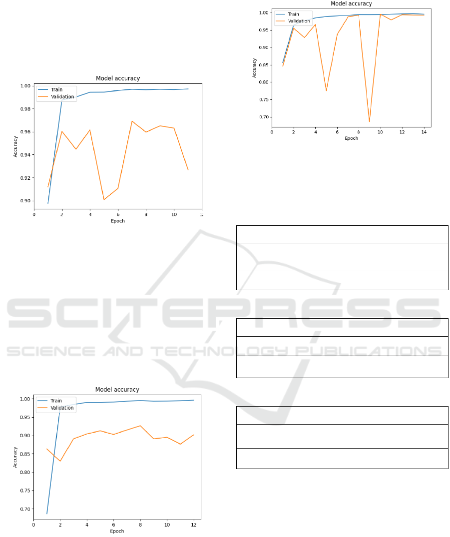
Fig. 2. shows the training process of models. For this

paper's convolutional neural network model, the

model was set to tolerate up to 4 training sessions that

failed to increase model accuracy. After training, the

model will return to its optimal state. This design can

ensure that the model has the best accuracy to a

certain extent.

Likewise, Fig. 3. and Fig. 4. indicate that these

models have been fully trained. Additional training can

lead to overfitting or the deterioration of accuracy.

Figure 3: Accuracy on datasets of model 2. under different

training times (Picture credit: Original).

Figure 4: Accuracy on datasets of model 3. under different

training times (Picture credit: Original).

3.2 Evaluation

Table 1: Result of model 1.

Accurac

Loss

Recall

Precisio

Trainin

0.9969

0.996

0.011

0.996

0.9971

Test

0.9692

0.969

0.220

0.968

0.9704

Table 2: Result of model 2.

Accurac

Loss

Recall

Precisio

Trainin

0.9953

0.995

0.018

0.995

0.9957

Test

0.9265

0.928

0.487

0.925

0.9318

Table 3: Result of model 3.

Accurac

Loss

Recall

Precisio

Trainin

0.9940

0.993

0.074

0.992

0.9949

Test

0.9949

0.995

0.065

0.994

0.9959

In the tables listed above, F1-score is abbreviated

as F1. The tables listed above demonstrated

differently in the test set. In this paper's fruit

classification context, the author believes that

comprehensively considering accuracy and f1-score

to evaluate the model's ability is the most appropriate

way to judge the models.

DAML 2023 - International Conference on Data Analysis and Machine Learning

364

Figure 5: Training Metrics. (Photo/Picture credit: Original).

Figure 6: Test Metrics. (Photo/Picture credit: Original).

From Fig. 5. and Fig. 6. although model 1. has the

best performance in its training, the performance of

its test is not the highest. Model 3. shows the worst

training accuracy but has the highest accuracy rate in

the test set.

4 DISCUSSION

Although model 1. has a relatively simple structure

and shallow layers, it still achieves rather good

recognition capabilities. However, although the

author designed model 2. with deeper layers to

improve its performance, it did not perform better

recognition results. After further deepening the

number, increasing its accuracy may become more

difficult. The author tried adding more layers to

model 2., but the model's accuracy remained small

and difficult to increase. The difficulty in training the

model may be due to a vanishing gradient. To confirm

this conjecture, the author used a residual neural

network because the residual neural network can

eliminate the training difficulty caused by excessive

depth by introducing linear transformation into the

nonlinear transformation. Although model 3. had

lower accuracy and f1-score and higher loss for the

training set, model 3. achieved the best accuracy in

the test set. For recognition situations that may

actually exist rather than fixed environments, such as

training sets, model 3. performs better than the

previous two models. This conclusion shows that

using residual neural networks is more effective than

simply adding convolutional neural network layers.

5 CONCLUSION

The residual neural network has better recognition

results with more layers, showing that the residual

neural network is more effective than the typical

convolutional network. Model 2. tries to improve the

network's performance by increasing the

convolutional layers, but it doesn't work. Model 3.

with residual blocks achieves the best accuracy and

f1-score in the research. Combining the performance

of the three models for data sets with smaller pixels,

using the residual network is more effective than

increasing the number of layers of the convolutional

neural network. The accuracy rate of approximately

99.5% can satisfy the needs of most fruit

classification conditions. However, this result only

represents theoretical feasibility. For example, fruit

images shot by cameras differ from the dataset used

in this article for the models, meaning more complex

data preprocessing steps are required. The fruit

classification and identification technologies still

need supporting physical equipment and further

experimental processes to prove their practicability in

agricultural production. At the same time, limited by

the data resolution size and quantity of the data set,

the model may not meet expectations when

processing actual inputs. In order to achieve better

recognition results, larger and more comprehensive

data sets are needed.

REFERENCES

A. B. Islam, “Machine Learning in computer vision,”

Applications of Machine Learning and Artificial

Intelligence in Education, pp. 48–72, 2022.

V. G. Dhanya et al., “Deep Learning Based Computer

Vision Approaches for Smart Agricultural

Applications,” Artificial Intelligence in Agriculture,

vol. 6, pp. 211–229, Sep. 2022.

Y. Chen et al., “Plant image recognition with Deep

Learning: A Review,” Computers and Electronics in

Agriculture, vol. 212, p. 108072, Sep. 2023.

Y. LeCun, Y. Bengio, and G. Hinton, “Deep learning,”

Nature, vol. 521, no. 7553, pp. 436–444, May 2015.

0,99200,99300,99400,99500,99600,99700,9980

model 1.

model 2.

model 3.

Training Metrics

Training F1-score Training Accuracy

0,9000 0,9200 0,9400 0,9600 0,9800 1,0000

model 1.

model 2.

model 3.

Test Metrics

Test F1-score Test Accuracy

Classiﬁcation of Fruits Based on Convolutional Neural Networks

365

S. Yu, S. Jia, and C. Xu, “Convolutional Neural Networks

for Hyperspectral Image Classification,”

Neurocomputing, vol. 219, pp. 88–98, Jan. 2017.

Y. Lecun, L. Bottou, Y. Bengio, and P. Haffner, “Gradient-

based learning applied to document recognition,”

Proceedings of the IEEE, vol. 86, no. 11, pp. 2278–

2324, 1998.

K. Simonyan and A. Zisserman, “Very deep convolutional

networks for large-scale image recognition,” arXiv.org,

2014 https://arxiv.org/abs/1409.1556.

S. Albawi, T. A. Mohammed, and S. Al-Zawi,

“Understanding of a convolutional neural network,”

2017 International Conference on Engineering and

Technology (ICET), Aug. 2017.

Y. Guo et al., “Deep Learning for Visual Understanding: A

Review,” Neurocomputing, vol. 187, pp. 27–48, Apr.

2016.

M. Tan and Q. Le, “EfficientNet: Rethinking Model

Scaling for Convolutional Neural Networks,” May

2019.

K. He, X. Zhang, S. Ren, and J. Sun, “Deep residual

learning for image recognition,” 2016 IEEE Conference

on Computer Vision and Pattern Recognition (CVPR),

Jun. 2016, pp. 770-778.

M. Oltean, “Fruits 360,” Kaggle,

https://www.kaggle.com/datasets/moltean/fruits

(accessed May 18, 2020).

DAML 2023 - International Conference on Data Analysis and Machine Learning

366