Urban Growth Modelling Based on CA-Markov Approach on

Bengaluru India

Jyothi Gupta

1 a

and Raghunandan Kumar

School of Architecture, CHRIST (Deemed to be University), Bengaluru, 560074, Karnataka, India

Department of Civil Engineering, CHRIST (Deemed to be University), Bengaluru, India

Keywords: Geospatial Modelling, Urban Growth Predictions, Cellular Automata-Markov Chain Model, Land Use / Land

Cover Change (LULC), Remote Sensing.

Abstract: The theme of this research is to create spatial patterns for Bengaluru city in India to understand the urban

growth over the past 40 years. The problem of our re-search addresses developing an integrated Geospatial

Modelling Approach to as-sess Urban Growth patterns in Bengaluru Metropolitan Region. This study uses

the various logical methods to create the Land Use/Land Cover (LULC) Map, all the datasets in google earth

engine are categorised in the Supervised Classification. Machine Learning Processes such as Random Forest

(RF), Classification and Regression Tree (CRT), and Support Vector Machine (SVM) classifiers are

considered for this Classification. The Classifier’s performance is evaluated using statistical measures like

overall Accuracy and kappa statistics. Classes with multiple parameters are carried out with the Hybrid

Cellular Automata- Markov (CA-Markov) method, which is capable of duplicating changes through one

grouping to another. This hybrid model supports model both spatial 3D and temporal time-based changes.

The main product after modelling predicts LULC for 2041 and 2051. The argument is that CA-Markov,

Shannon entropy will allow us to define how much area of all classes will be changed in 2041 and 2051.

1 INTRODUCTION

Land use is a phrase that is referred to how humans

use the land and its resources, as well as the purposes

for why they do so. The environment or vegetation

type present, like forests or farmland, is referred to as

land cover. Artificial changes in the earth's crust are

referred to as land use/land cover (LULC), often

called land change (Bhat et. al, 2015). Landcover use

has been identified as a fundamental cause of climatic

change on geographical and time dimensions,

appearing as a critical environmental concern and one

of the major research initiatives on global change

research on a local scale (Baqa et al, 2021).

2 AIM AND OBJECTIVES

AIM: To develop a cohesive CA-Markov Model

Approach to assess Urban Growth patterns in

Bengaluru Metropolitan Region.

https://orcid.org/0000-0003-0612-0188

Objective of the Study: Visualize and analyse the

Spaciotemporal transformation in Land use /Land

cover (LULC) from -1991,2001,2011,2021(40

years). Simulate the past LULC and forecast the

future development of the Bengaluru Metropolitan

Region using CA Markov Model 2031, 2041.

Identifying Specific Regions where intense Urban

Growth can occur in Bengaluru Metropolitan Region.

Table 1: Methodology Flow using Google earth engine.

Google

earth engine

(GEE)

Export

Landsat

images in

tiff format

Creating

train/test

data for

class

Use of

Classifier

Train the

classifier

using train

data

Classify as

image or

feature

selection

Data

catalog

DEM

OSM

Data

(Road

layer)

Landsat 5,7

and

Sentinel

-2

Data from

Slope,

Aspect

Euclidean

distances

On roads

and Urban

Image pre

processing

LULC

change

analysis

LULC

change

matrix

Supervised

LULC

Transition

Potential

Transition

Potential

Map

Reference

Maps

Gupta, J. and Kumar, R.

Urban Growth Modelling Based on CA-Markov Approach on Bengaluru India.

DOI: 10.5220/0012876600003739

Paper published under CC license (CC BY-NC-ND 4.0)

In Proceedings of the 1st International Conference on Artiﬁcial Intelligence for Internet of Things: Accelerating Innovation in Industry and Consumer Electronics (AI4IoT 2023), pages 385-391

ISBN: 978-989-758-661-3

385

classificatio

Modelling

(MLP)

Accuracy

Assessment

91,2001,21,

CA Markov

Simulation

Model

Validation

for 21

Calibrated

Markov

Model 31-

Predicted

LULC maps

The table 1 shows the flow in methodology, which

is used in this study.

3 DATA COLLECTION

The Remote Sensing Data of LANDSAT

Multispectral, TM, ETM+, and OLI/TIRS &

Sentinel-2 MSI: Multispectral Instrument, Level-2A

data is used for Supervised Classification such as

Random Forest (RF), Classification and Regression

Tree (CRT), and Support Vector Machine (SVM) in

Google Earth Engine (GEE). Using these datasets,

land use land cover (LULC) for

1991,2001,2011,2020 are Simulated in Google Earth

Engine. Digital Elevation Model (DEM) from Earth

Data by NASA is Downloaded in table 1-2. The

Digital Elevation Model (DEM) Slope is Generated

in ArcGIS Pro. The Slope gives the identification of

terrain, whether the Terrain is Steep or flat (Mishra et

al, 2014). The low slope value will have flat terrain,

and a high slope value will have steep terrain. From

the Slope, the aspect is generated. The aspect

identifies the downscale direction of a high-value

change rate through one cell towards its neighbours.

Road Layer has been obtained from the Open Street

map. Euclidean Distance to Roads and Railways are

Considered. Euclidean Distance to Built-up is also

considered. Table 2 is created to show the link

attachment.

Table 2: Data collection from Online link.

Year

Data

GEE Spatial resolution / Link

1991

Landsat 5 Series

TM AND ETM -

GEE

30 m

2001-2011

Landsat 7 Series

TM AND ETM -

GEE

30 m

2021

Sentinel – 2 GEE

datasets

10m to 60 m

Administrative and

city boundary

Shapefile-https://www.diva-

gis.org/

DEM (Digital

Elevation/Terrain

model) for Slope

and Aspect

Earth Data -

https://earthdata.nasa.gov/

Census data for 4

decades

Census of India

https://censusindia.gov.in/

Road network and

Railway

Open Street Map

https://www.openstreetmap.org/

4 CA-MARKOV MODEL

The CA-Markov model a hybrid model which

develops the traditional Markov model with the

Cellular Automata model (CA). The CA methods are

utilized to regulate the spatial dynamics of the GIS

platform (Jain et al, 2016). The spatiotemporal raster

Based da-ta modelling is employed to show what has

changed for constant data over time across Land

use/land cover categories using transition probabilities.

When it comes to land-use change projections, the

Markov model concentrates upon quantity (Jadawala

et al, 2021). The spatial parameters of this model are

inadequate and don't account for the different forms of

land use types of variations in the spatial magnitudes.

The CA model prepares a robust area conception; this

means it can handle complex space systems in terms of

space-time dynamic evolution (Yadav et al, 2021). The

CA–Markov model, which combines Markov and CA

theories, is concerned with time series and space for

prediction purposes. This could effectively simulate

changes in quantity and space of land use patterns

throughout time and space. The LULC maps were

created using the Google Earth engine, then exported

as Geo Tiff files and divided into four categories.

Water is in class 1, Vegetation is in class 2, Barren is

in class 3, and Built-up is in class 4. These LULC maps

were converted into rst format from Geo Tiff Format

in Clark Labs TerrSet IDRISI software. The land

change modeller(figure1-3) helps to make the forecast

LULC diagram centred on equally the previous LULC

map and future LULC plan.

This panel in figure 1 creates several Transitional

maps. Changes, persistence, gains, and losses can be

mapped by land use/cover class, as well as transitions

and transfers by class. Change patterns in

environments influenced by hu-man intervention can

be complex and challenging to recognize. A

geographic trend analysis tool was developed to aid

understanding in such circumstances. This is the

polynomial trending surface that best fits the

changing pattern. A call to a TREND module

analyzes this choice as show in figure 1a.

To Predict 2031 & 2041 Land Use Land Cover,

Clark Labs TerrSet IDRISI software was employed in

2 ways to build transition areas & transition area

probability matrices.

For LULC change analysis, the Land use/Land

cover Change module software Land Change Modeler

(LCM) is employed. The Change Module investigates

the difference among two LULC photos, namely the

previous and latter land cover photographs as show in

in figure 1b. All the Parameters should be converted to

AI4IoT 2023 - First International Conference on Artiﬁcial Intelligence for Internet of things (AI4IOT): Accelerating Innovation in Industry

and Consumer Electronics

386

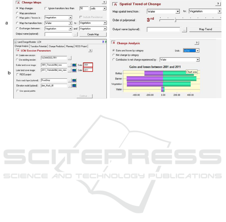
Figure 1: (a) Changes in map and Spatial trends and (b) Change analysis’s and LCM parameters.

rst for-mat from Geo-tiff Format in Land Change

modeler.

Clark Labs TerrSet IDRISI software will estimate

LULC parameters based on previous and current

Land use/land maps to generate Change possibility

matrix reports that reflect the chance of both LULC

class transitioning to alternative session.

Secondly, a CA-Markov model has helped to

forecast the Transition in the LULC categories for

2031 and 2041. Additionally, with the use of two

LULC maps created from satellite photographs. The

model is used to determine the set of a random

process, X (t), at every point in time-period, t1, t2,

tn,tn + 1; consequently, the unplanned processes will

explain in equation 1.

(()) = , ( − 1) =  − 1, (1) =

(()) =  (1)

tn shows the present time and tn+1 denotes time in

future; t1, t2, t3, t4……, tn − 1 implies continuous

time frame moments in the previous time. According

to current realities, the future remains independent of

the previous time. Hence, the future random process

is not affected by someplace it occurs. It is not where

it used to be or where it is today. If M[k] is the

Markov chain, and xn is a group of N states (x1, x2,

x3…... xn), The chance of Transition between

condition i to condition j for single time instant is

given by Equation 2.



.





(



[

 + 1

]

= 



[



]

= 

)

(2)

The Land Change Modeler module provides three

techniques for constructing transition potential maps

associated with sub- models and independent

Parameters: a multi-layer perceptron (MLP) neuronic

network link, logistic regression, and a machine

learning tool like similarity -weighted instance (Sim-

Weight). The MLP correctly forecasts the plot that will

transfer since the picture of a subsequent stage to the

indicated simulated period, depending on the

projections. MLP surpasses alternative strategies in

estimating the correlation among nonlinear land-use /

land cover LULC changes and explanatory variables in

equation 3-4. When several transition types are

modeled, it is more versatile and dynamic than the

others.

( + 1) = 



× () (3)

where 0 ≤ Pij < 1 and n ∑ j=1 Pij = 1, (i, j = 1, 2, . .

., n).

The following formula is used to definite the CA

cellular automata model:

(,  + 1) = [(), ] (4)

where S(t) and S(t+1) are the organization rank at

periods t and t + 1, correspondingly. N represents the

cellular field, t, t + 1 represent distinct intervals, f

symbolizes the transforming rule of cellular conditions

in a particular region, S represents the group of

restricted and distinct cellular conditions, and Pij

represents the evolution probabilities in a phase.

5 SHANNON ENTROPY (HN)

Shannon Entropy is a commonly used metric of

spatial dispersion or concentration that is widely used

in the research of the urban sprawl phenomenon. The

Hn measurement depends on the entropy concept,

which was first designed to quantify information. It is

a valuable and dependable metric for deciding the

level of compactness & dispersion of urban

expansion.

Urban Growth Modelling Based on CA-Markov Approach on Bengaluru India

387

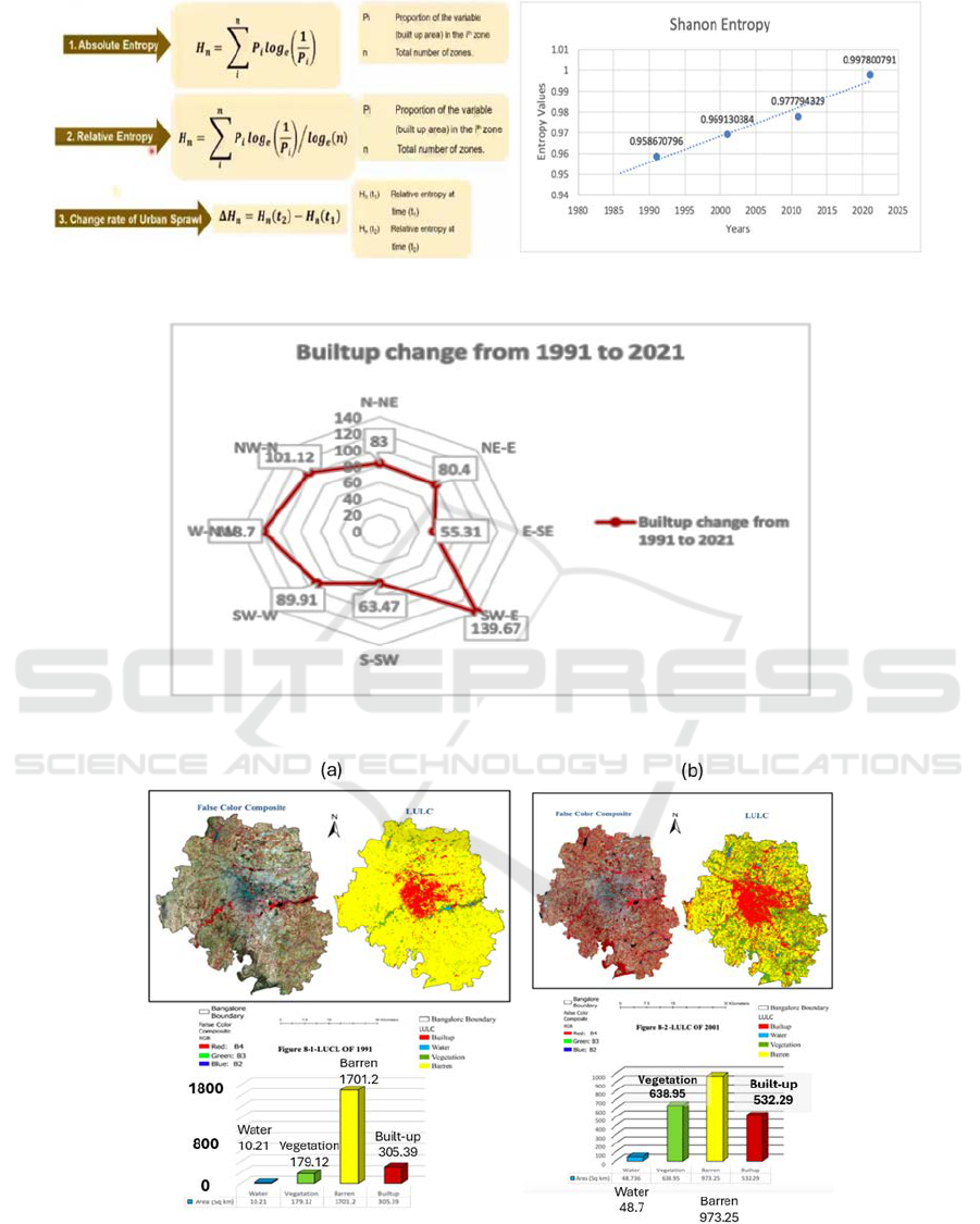
Figure 2: Shannon Entropy Equation & Obtained results.

Figure 3: Built-up changes and Line graph for Shannon Entropy.

Figure 4: Spatial Urban pattern LULC showing growth (a) 1991, (b) 2001,2022,2021.

AI4IoT 2023 - First International Conference on Artiﬁcial Intelligence for Internet of things (AI4IOT): Accelerating Innovation in Industry

and Consumer Electronics

388

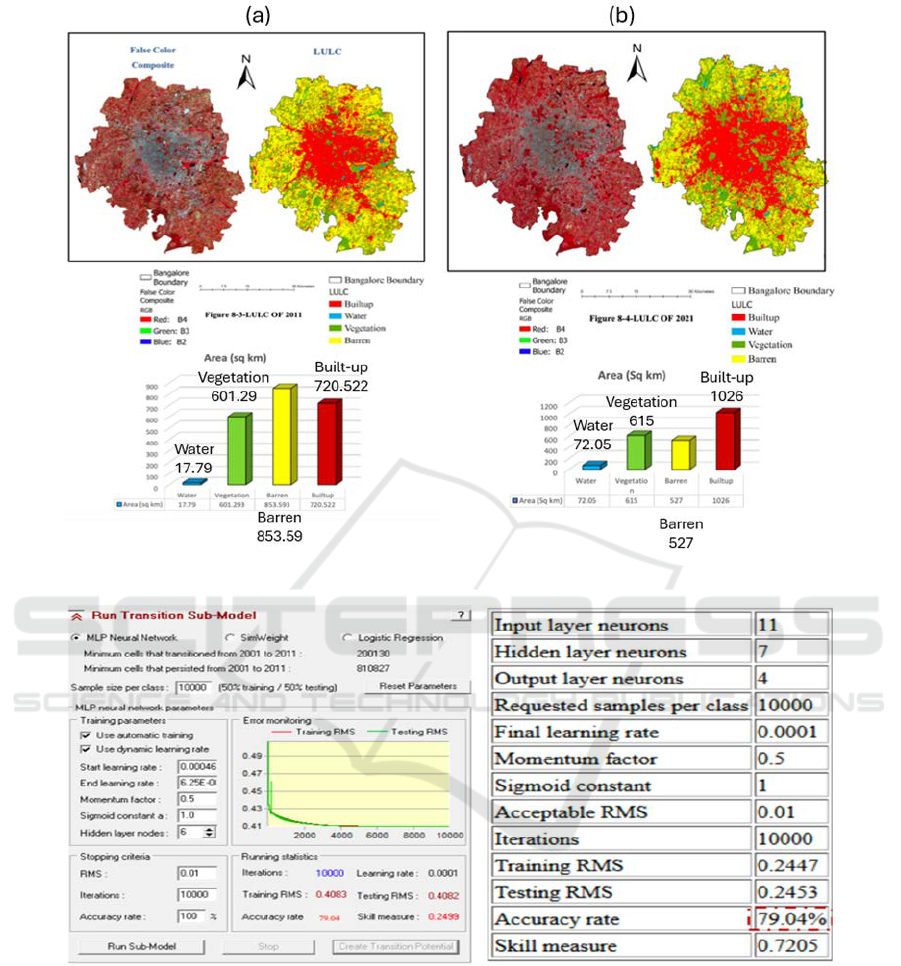
Figure 5: Spatial Urban pattern LULC showing growth (a) 2021, (b)2022.

Figure 6: Model Accuracy.

Urban Growth Modelling Based on CA-Markov Approach on Bengaluru India

389

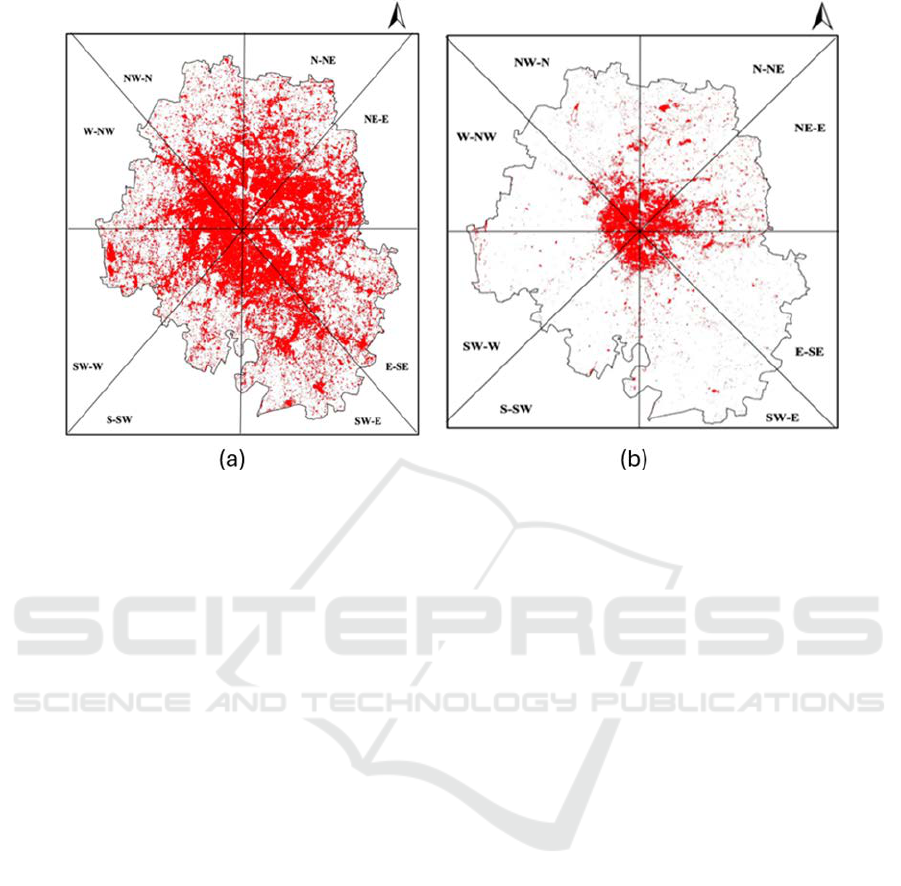
Figure 7: Bangalore Builtup area (a) 2001 (b) 1991.

Where Pi is the fraction of a geophysical

parameter in i-th zone and n symbolises the overall

sum of zones as seen in figure 2. The entropy value

can range amid 0 and log (n). A number around 0

implies a relatively tight circulation, while a value

close to log(n) show a scattered distribution. The mid-

level of log(n) is regarded as the threshold level;

hence, a city with just an entropy value higher than

the threshold value is referred to be a spreading city.

From 1991 to 2021, the most significant shift has

occurred in the Southeast direction, where the Built-

up area has urban growth as shown in figure 3-4.

We can see the Spatial Change patterns of

Bengaluru’s significant barren land from 1991 and

how it changed to a built- up area in 2021 due to urban

sprawl. We can see the patterns of change analysis of

how vegetation increased from 1991 to 2021 and how

it progressively reduced and then rose. Gains and

losses, change transitions, and change analysis are

patterns we've seen where substantial barren land has

been turned into Urban land.CA Markov is the most

common and effective modeling method for many

researchers who often use for modeling urban growth.

We forecasted forthcoming LULC land use/land

cover for 2031 and 2041 using the CA-Markov

model, and we have calculated the future Area in sq-

km of all classes. Which will aid in identifying where

and in which direction built up would increase and

which city planners can use to prepare for future

expansion.

The dynamic learning process begins with a

strong learning rate but decreases gradually over

repetitions till the last knowledge proportion is

stretched at what time the highest sum of repetitions

is extended. If a huge fluctuation in the RMS

inaccuracy is found during the first number of

reiterations, the learning rates (begin and finish) are

condensed by part, and the technique is repeated in

figure 6. LCM keeps the MLP's (Multi-layer

Perception) other variables at their default settings.

On the other hand, LCM does not make any specific

changes to outputs. Because changes are being

simulated, LCM filters out any circumstances that do

not meet the context of any given transition from the

transitional potentials. In figure 3 if the change is

from Barren to Vegetation, values will only occur in

a pixel before Barren, then Transition potential maps

are generated. The dynamic learning process begins

with a strong learning rate but decreases gradually

over repetitions till the absolute learning rate is

extended once the extreme sum of iterations is gotten.

If a enormous fluctuation in the RMS mistake is

found during the first number of iterations, the

absorbing charges (begin and finish) are abridged by

quasi, and the procedure is repeated. LCM keeps the

MLP's (Multi-layer Perception) other variables at

their default settings. On the other hand, LCM does

not make any specific changes to outputs. Because

changes are being simulated, LCM filters out any

circumstances that do not meet the context of any

given transition from the transitional potentials. In

AI4IoT 2023 - First International Conference on Artiﬁcial Intelligence for Internet of things (AI4IOT): Accelerating Innovation in Industry

and Consumer Electronics

390

figure 7 if the change is from Barren to Vegetation,

values will only occur in a pixel before Barren, then

Transition potential maps are generated.

In 1991, Barren Land accounted for around 75 %

of the overall Bengaluru District Boundary, while

Vegetation accounted for 9.2 %, and built-up area

accounted for 15 % of the total Bengaluru District

Boundary. Then, in 2001, we can see that bare land

decreased to 30.7 %, while built-up has expanded 9.2

% since 1991 and Vegetation rose exponentially to

29.2 %. Between 2001 and 2011, barren land was

reduced by 8%, and Vegetation was decreased by 4%,

resulting in an 8.2% increase in an urban area in 2011

as barren plot was transformed into the urbanized

area. From 2011 to 2021, barren land was reduced by

14.81%, and Vegetation has been increased by 2%,

resulting in a 13.9 % increase in an urban area in 2021

(figure 5-7).

Because the Accuracy of the Land Change

Modeler is 79.02 percent, we can claim it will predict

about 80 percent of the time. As shown, Bengaluru’s

future urban growth and the direction in which the

city is expanding are visible.

Between 2021 and 2031, bare land will be reduced

by 5.78%, and Vegetation will be reduced by 4%,

resulting in a 7.88% increase in urban areas in 2031.

The total built-up area will increase by 54.6 %.

Between 2031 and 2041, bare land will be reduced by

4 %, and Vegetation will be reduced by 2%, resulting

in a 6.4 % increase in urban areas in 2041. The total

built-up area will increase by 61 %.

6 CONCLUSIONS

Using Shannon Entropy, we can see that the most

substantial change from 1991 to 2021 happened in the

Southeast direction, where the Built-up region has

increased. This study concludes the challenges and

issues of urbanization in Bengaluru (Gupta J, 2022).

The solutions to these concerns are GIS data and

raster data are employed. Raster data are collected

from the google earth engine & GIS Data are gathered

from different web portals & studied various research

literature in the journal about the problem. To bring

this study to a close, qualitative, and quantitative tools

were examined. This paper explains the logical

method, which must be associated with the CA

Markov Model and the Shannon Entropy Study.

This report requires Future research of

Bengaluru’s changing spatial patterns of urban

growth. It is challenging to identify significant

differences between agriculture and parks because of

the low spatial resolution of Landsat 5 & 7 (Gupta et

al, 2015). The CA Markov model has a drawback in

that it cannot be employed for short time intervals.

While calibration is the most crucial procedure for

determining which parameters are appropriate for the

model, this model has been run more than 15 times.

Each time the parameters change, the results vary.

REFERENCES

Bhat, V., Aithal, B. H., & Ramachandra, T. V. (2015).

Spatial patterns of urban growth with globalisation in

India’s Silicon Valley. Organized By Department of

Civil Engineering, Indian Institute of Technology

(Banaras Hindu University), Varanasi-221005 Uttar

Pradesh, India, 98.

Baqa, M. F., Chen, F., Lu, L., Qureshi, S., Tariq, A., Wang,

S., ... & Li, Q. (2021). Monitoring and modeling the

patterns and trends of urban growth using urban sprawl

matrix and CA-Markov model: A case study of

Karachi, Pakistan. Land, 10(7), 700.

Mishra, V. N., Rai, P. K., & Mohan, K. (2014). Prediction

of land use changes based on land change modeler

(LCM) using remote sensing: A case study of

Muzaffarpur (Bihar), India. Journal of the

Geographical Institute" Jovan Cvijic", SASA, 64(1),

111-127.

Jain, S., Siddiqui, A., Tiwari, P. S., & Shashi, M. (2016).

Urban growth assessment using CA Markov model: A

case study of Dehradun City. 9th International

Geographic Union.

Jadawala, S., Shukla, S. H., & Tiwari, P. S. (2021). Cellular

automata and markov chain based urban growth

prediction. International Journal of Environment and

Geoinformatics, 8(3), 337-343.

Yadav, V., & Ghosh, S. K. (2021). Assessment and

prediction of urban growth for a mega-city using CA-

Markov model. Geocarto International, 36(17), 1960-

1992.

Gupta, J. (2022, November). Statistical Assessment of

Spatial Autocorrelation on Air Quality in Bengaluru,

India. In International Conference on Intelligent Vision

and Computing (pp. 254-265). Cham: Springer Nature

Switzerland.

Gupta, A. J., & Subrahmanian, R. R. Design Challenges of

Project Deliverables in Construction Industry in

Bangalore.

Urban Growth Modelling Based on CA-Markov Approach on Bengaluru India

391