Graph Convolutional Networks for Image Classiﬁcation: Comparing

Approaches for Building Graphs from Images

ulia Pelayo Rodrigues

and Joel Lu

ıs Carbonera

Institute of Informatics, Federal University of Rio Grande do Sul, Porto Alegre, Brazil

Keywords:

Graph Neural Networks, Image Classiﬁcation, Superpixels, Graph Convolutional Networks.

Abstract:

Graph Neural Networks (GNNs) is an approach that allows applying deep learning techniques to non-euclidean

data such as graphs and manifolds. Over the past few years, graph convolutional networks (GCNs), a speciﬁc

kind of GNN, have been applied to image classiﬁcation problems. In order to apply this approach to image

classiﬁcation tasks, images should be represented as graphs. This process usually involves over-segmenting

images in non-regular regions called superpixels. Thus, superpixels are mapped to graph nodes that are char-

acterized by features representing the superpixel information and are connected to other nodes. However,

there are many ways of transforming images into graphs. This paper focuses on the use of graph convolutional

networks in image classiﬁcation problems for images over-segmented into superpixels. We systematically

evaluate the impact of different approaches for representing images as graphs in the performance achieved by

a GCN model. Namely, we analyze the degree of segmentation, the set of features chosen to represent each su-

perpixel as a node, and the method for building the edges between nodes. We concluded that the performance

is positively impacted when increasing the number of nodes, considering rich sets of features, and considering

only connections between similar regions in the resulting graph.

1 INTRODUCTION

Graph Neural Networks (GNNs) (Scarselli et al.,

2009)) is an approach that generalizes neural net-

works, allowing them to deal with non-euclidean data

such as graphs. This capability of dealing with graphs

as inputs makes it possible to apply deep learning ap-

proaches to a vast set of problems whose data can

be modeled as graphs. Since they were proposed,

GNNs have been applied in different areas (Wu et al.,

2020), such as Bioinformatics (Zhang et al., 2021),

Particle Physics (Shlomi et al., 2020), Neuroscience

(Bessadok et al., 2022), natural language processing

(Wu et al., 2023), material science and Chemistry

(Reiser et al., 2022), Computer vision (Chen et al.,

2022; Todescato et al., 2024), etc.

In the last few years, several studies have inves-

tigated how to apply GNNs for image classiﬁcation

(Hong et al., 2020; Chen et al., 2020; Zhang et al.,

2023; Du et al., 2023; Tang et al., 2022). Most of

these studies are based on a speciﬁc type of GNN

called graph convolutional network (GCN) (Kipf and

Welling, 2017), which can be understood as a gener-

https://orcid.org/0009-0003-0821-4281

https://orcid.org/0000-0002-4499-3601

alization of convolutional neural networks to graph-

structured data.

In order to apply GNNs for classifying images,

it is necessary to represent the image information as

a graph. Typically, these approaches involve over-

segmenting images into non-regular regions called su-

perpixels (Defferrard et al., 2016; Monti et al., 2016)

that are mapped to nodes in a graph. However, in

this approach, there are different ways of building the

resulting graph, depending on choices made by the

designer on different aspects. For example, the im-

ages can be segmented in different degrees, resulting

in different numbers of nodes in the graph and in dif-

ferent densities of pixels per node. Besides that, there

are different approaches for deﬁning the edges among

the nodes that represent superpixels, such as adopt-

ing fully connected graphs (Monti et al., 2016), K-

Nearest Neighbors, region adjacency graphs (Avelar

et al., 2020a), dynamic approaches (Linh and Youn,

2021), etc. Furthermore, there are different ways of

assigning features to nodes in order to represent the

superpixels’ features in the original image.

However, as far as we are aware, the literature

does not provide any systematic comparison of how

different ways of building graphs impact the per-

Rodrigues, J. and Carbonera, J.

Graph Convolutional Networks for Image Classiﬁcation: Comparing Approaches for Building Graphs from Images.

DOI: 10.5220/0012263200003690

Paper published under CC license (CC BY-NC-ND 4.0)

In Proceedings of the 26th International Conference on Enterprise Information Systems (ICEIS 2024) - Volume 1, pages 437-446

ISBN: 978-989-758-692-7; ISSN: 2184-4992

437

formance achieved by GCNs in image classiﬁcation

tasks. Such systematic evaluation would be a valuable

reference for supporting the most effective choices

when designing models in this context.

In this paper, we focus on using Graph Convo-

lutional Networks (Kipf and Welling, 2017) (GCNs)

for the classiﬁcation of superpixel segmented images

using the SLIC (Achanta et al., 2012) method in its

adaptive (SLICO) variant. Our objective is to system-

atically evaluate the impact of the following graph-

building choices on the performance of a simple GCN

model: (I) the degree of segmentation (that deﬁnes the

number of nodes in the resulting graph); (II) the selec-

tion of features for characterizing each node, and rep-

resenting the superpixels’ information; and (III) the

method for deﬁning edges between node pairs in the

resulting graph.

We have found that the performance achievable by

the GCN model is positively impacted by choosing

rich representative feature sets, increasing the num-

ber of superpixels per image – although the positive

impact grows smaller as the number of pixels per su-

perpixel approaches one –, and by building neighbor-

hoods between nodes that encompass only similar re-

gions (that is, considering descriptive features in the

calculation of the distance between nodes and limit-

ing the maximum degree).

The remainder of this paper is structured as fol-

lows. In Section 2 we discuss the related work. In

Section 3 we present our experiments and discuss our

results. Finally, Section 4 presents the conclusions.

2 RELATED WORKS

Errica et al. (Errica et al., 2022) have compared dif-

ferent GNN architectures’ (including GCNs) perfor-

mance in the task of graph classiﬁcation, drawing

attention to the reproducibility problems present in

the literature. They propose a rigorous method for

model evaluation and comparison – highlighting the

importance of using the same features and number of

nodes – and a standardized and reproducible experi-

mental setting. They are also able to establish, using a

structure-agnostic baseline model, that not always are

GNNs able to take advantage of the structural infor-

mation in graphs.

Shchur et al. (Shchur et al., 2019) also point

out limitations in the empirical evaluation process of

GNN models, focusing on node classiﬁcation tasks.

They discuss the effects of train/test/validation dataset

splits on performance, ﬁnding that with the same hy-

perparameter selection and training procedures sim-

ple GCNs may be able to outperform more sophisti-

cated models.

Xu et al. (Xu et al., 2019) provide a theoretical

analysis of the representative power of different GNN

models – in addition to proposing their own model,

the Graph Isomorphism Network (GIN) – and exper-

imentally compare them using different graph classi-

ﬁcation datasets, showing that, in most cases, more

representative power implies greater accuracy.

Monti et al. (Monti et al., 2016) introduced the

MoNet framework for generalizing CNN architec-

tures to graphs and manifolds. They also proposed a

model that was applied to, among other tasks, image

classiﬁcation, using both uniform grids and SLIC su-

perpixels as segmentation methods. In the superpixel

approach the graphs were fully connected, while in

the grid approach, each node was connected to its im-

mediate and diagonal neighbors, with grids yielding

better results. No references are made regarding the

method used for building node features.

Avelar et al. (Avelar et al., 2020b) used Graph At-

tention Network (GAT) for superpixel image classiﬁ-

cation. Their method consists of segmenting the input

image into superpixels using the SLIC method, ex-

tracting features (namely average color and centroid,

although other options are also suggested) from them,

and building region adjacency graphs. The resulting

graph is then fed into the GAT. They concluded that

GAT networks are not able to achieve the same per-

formance achieved by more sophisticated models.

Long et al (Long et al., 2021) proposed the Hi-

erarchical GNN (HGNN) with multiple GAT layers,

aggregating each layer’s output. The method was ap-

plied to superpixel image classiﬁcation. The graph

was built with SLIC superpixels as nodes, with aver-

age color and centroid as features. The edges were

built with a K-Nearest Neighbors approach, using as

the distance metric the average distance of each color

channel and spatial dimension.

Linh et al. (Linh and Youn, 2021) proposed

the Dynamic Superpixel Cloud GCN (DISCO-GCN)

model, using GCN layers with edges generated dy-

namically before each layer. They also use SLIC su-

perpixel segmentation, building features using only

color information, although they also suggest the pos-

sibility of spatial features (such as the centroid).

As far as we are aware, the literature does not

provide any systematic comparison of how differ-

ent ways of building graphs impact the performance

achieved by GCNs in image classiﬁcation tasks.

ICEIS 2024 - 26th International Conference on Enterprise Information Systems

438

3 EXPERIMENTS

In this Section, we systematically analyze the impacts

on the performance of an image-classiﬁcation GCN

model of different methods for building

graphs that

represent images. We evaluated three dimensions of

the graph-building process: node features, number of

nodes, and edge-building method.

In each experiment, the following datasets were

used: MNIST (Lecun et al., 1998), Fashion-MNIST

(Xiao et al., 2017), CIFAR-10 (Krizhevsky, ), CIFAR-

100 (Krizhevsky, ), and STL-10 (Coates et al., ). All

datasets are balanced (with the same number of im-

ages for each class). In each dataset, all images have

a homogeneous size. Other characteristics of the se-

lected datasets are described in table 1.

For extracting superpixels from images, we

adopted the SLIC method (Achanta et al., 2012) in its

adaptive (SLICO

) variant. The difference between

SLIC and SLICO is in the input parameters: SLIC re-

quires the user to input both the approximate number

of superpixels to create and the compactness factor,

and SLICO only needs the number of superpixels. In

this context, compactness is a measure of shape cal-

culated as a ratio of the perimeter to the area. Thus,

SLICO adaptively changes the compactness factor

depending on the texture of the region, resulting in

regularly shaped superpixels regardless of the tex-

ture (Yassine et al., 2018). Several other approaches

for extracting superpixels are also available, such as

SEEDS (Van den Bergh et al., 2015), SNIC (Achanta

and Susstrunk, 2017) and ETPS (Yao et al., 2015).

However, SLIC is preferred among most other state-

of-the-art methods (Stutz et al., 2018) and is readily

available in both of its considered variants. Besides

requiring just a single parameter, SLICO also tends

to produce more stable segmentation results, with re-

spect to the effective number of pixels compared to

n. It is important to note that the implementation of

the SLICO method adopted in this work only admits

superpixels composed of a minimum of 2 pixels, lim-

iting thus the number of nodes that can be generated.

It is also noteworthy that, given the n parameter that

deﬁnes the desired number of superpixels to be ex-

tracted from the image, it is not guaranteed that the

SLICO method will produce exactly n superpixels.

For training the GCN model, the Adam optimizer

was used, with a ﬁxed learning rate of 0.0001, and

The source code developed for building graphs from

images, can be found in https://github.com/BDI-UFRGS/

superpixel-graphs

We adopted the OpenCV implementation of SLICO,

whose documentation can be found in https://docs.opencv.

org/3.4/df/d6c/group ximgproc superpixel.html

cross entropy loss. We adopted a stratiﬁed 5-fold

cross-validation procedure, and every result reported

henceforth is the average of the ﬁve folds. In each

fold, one-ﬁfth of the dataset is used as test data, and,

of the remaining 80%, 10% is used for validation

and 90% training, respecting class distributions. We

adopted accuracy and macro f1-measure as perfor-

mance metrics. There are 100 training epochs, and

the ﬁnal model is the one with the greatest validation

f1-measure.

In the following sections, we present the GCN

model used in our experiments and, after, we describe

each experiment and its results.

3.1 The Model

The model used in the following experiments con-

sists of a group of sequential GCN layers, each fol-

lowed by a ReLU activation layer. This sequence of

layers is followed by a global mean pooling and a

global max pooling operation, both resulting in vec-

tors r ∈ R

|F|

, where |F| is the number of features that

characterize each node. The global max pooling op-

eration computes the feature-wise maximum values

across the nodes of the graph, and the global mean

pooling computes the feature-wise mean. The two

vectors resulting from these operations are concate-

nated and passed through a fully connected layer with

linear activation, with the output given by the follow-

ing softmax module. The model is illustrated in Fig.

To determine the number of GCN layers for the

model used in our experiments, we evaluated the

impact that different quantities have on the model’s

performance considering a ﬁxed graph generation

method. For each dataset, we considered models with

1, 2, 3, and 4 GCN layers. We used region adjacency

graphs (where nodes are connected considering all the

adjacent neighbors of each superpixel in the original

image) with approximately 75 nodes and average and

standard deviation of color, geometric centroid, and

standard deviation from centroid as features.

As can be seen in Figure 2, except for MNIST –

the simplest dataset in the selection – raising the num-

ber of layers to four, at best, has little effect on the

performance when compared with the three-layered

model and, at worst, decreases the performance (as

is the case of CIFAR-10 and STL-10). However, in

most datasets, raising the number of layers from two

to three results in performance gains. Based on these

results, we used three sequential GCN layers for the

experiments described in the following sections.

Graph Convolutional Networks for Image Classiﬁcation: Comparing Approaches for Building Graphs from Images

439

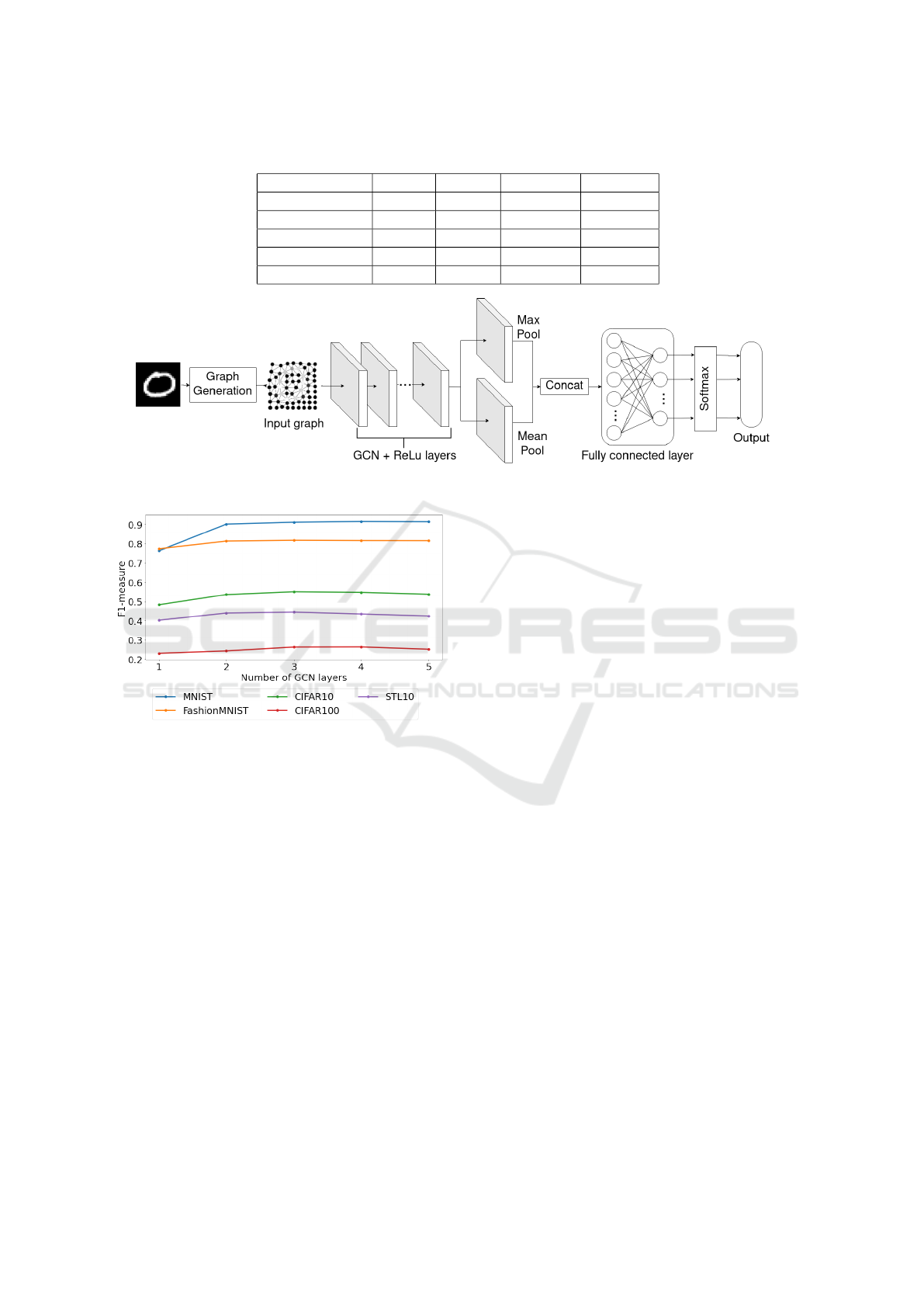
Table 1: Dataset characteristics.

Dataset Images Classes Color Area (px)

MNIST 70000 10 Greyscale 28x28

FashionMNIST 70000 10 Greyscale 28x28

CIFAR10 60000 10 Color 32x32

CIFAR100 60000 100 Color 32x32

STL10 13000 10 Color 96x96

Figure 1: Diagram representing the model’s architecture.

Figure 2: Test F1-measure with macro average w.r.t. the

number of GCN layers.

3.2 Evaluating Node Features

In our ﬁrst experiment, we evaluated how node-

feature selection impacts model performance. In or-

der to do that, we considered the following possible

features, all extracted from spatial and color (RGB or

greyscale, depending on the particular dataset’s char-

acteristics) information of the pixels that compose

each superpixel extracted from the original image by

the SLICO method:

• Geometric centroid: average 2D pixel position in

the original image;

• Standard deviation of pixel positions from the

centroid;

• Number of pixels: total number of pixels, or pixel

density, in the superpixel;

• Average RGB color: average R, G, and B values

in colorful datasets or average greyscale value in

greyscale datasets;

• Standard deviation from average color: standard

deviation of R, G, and B mean values in color

datasets or of greyscale mean value in greyscale

datasets;

• Average HSV color: only used in color datasets

(i.e. CIFAR-10, CIFAR-100, and STL-10), aver-

age values in HSV color space;

• Standard deviation from average HSV color: only

used in colorful datasets, the standard deviation of

values in HSV color space.

Our method consisted of selecting an initial base-

line feature vector containing only one feature and

then progressively expanding the baseline by adding

new features, analyzing how each increment impacted

the model’s performance. We selected as the baseline

feature the average color (RGB in colorful datasets,

greyscale otherwise), which is the feature most com-

monly used in the literature, to the best of our knowl-

edge. That is a one-dimensional feature vector in

greyscale datasets and a three-dimensional vector in

colorful datasets. The order in which the remaining

features were added was, from ﬁrst to last: geometric

centroid, standard deviation of color, standard devia-

tion of centroid, and number of pixels. For colorful

datasets were also added, in that order: average HSV

color, and standard deviation of HSV color.

In this experiment, we used the SLICO algorithm

for segmentation, with parameter n, the desired num-

ber of superpixels, ﬁxed at 75. For deﬁning the edges

of the resulting graph, we adopted region adjacency

graphs.

Figure 3 shows the evolution of the macro f1-

ICEIS 2024 - 26th International Conference on Enterprise Information Systems

440

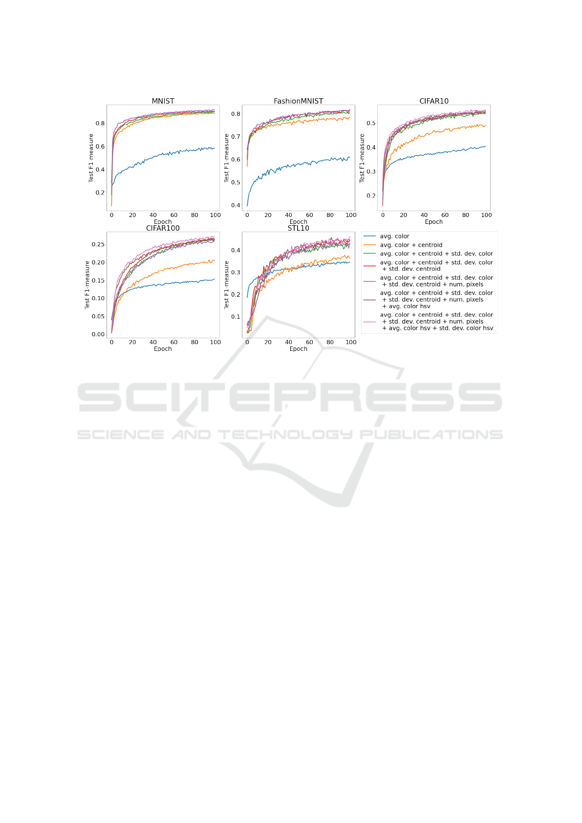
Figure 3: Test F1-measure with macro average along training process for each dataset in the experiment.

measure of the test set over the 100 epochs and Ta-

ble 2 presents the ﬁnal accuracy and f1-measure on

the test set achieved by the model for each dataset

and feature added to the progressively built baseline

feature vector. Our results suggest that the most sig-

niﬁcant performance gain is obtained when adding

to the baseline RGB/greyscale color information the

spatial information from the centroid. But, also, a

consistent improvement is seen when adding the stan-

dard deviation of RGB/greyscale color. The inclusion

of the standard deviation from the centroid resulted

in performance improvements, especially in MNIST,

FashionMNIST, and STL-10 datasets. Our results

also suggest that the performance can be improved by

adding average color and standard deviation values in

different color spaces to compensate for the loss of in-

formation that comes with the segmentation process.

3.3 Evaluating the Number of Nodes

Another important choice when building the image

graph is determining the number of nodes, which, in

this case, and in most superpixel approaches, is di-

rectly related to the number of superpixels generated

in the segmentation process. That corresponds to, in

this particular work, choosing the value of the de-

sired number of superpixels parameter – henceforth

referred to as n – in the SLIC algorithm variations.

Here, once more, region adjacency graphs were

used and the node features selected, as described in

the previous subsection, were: average color, geo-

metric centroid, standard deviation of RGB/greyscale

color, and standard deviation of centroid (the best-

performing features that are also applicable to all

datasets).

Our method consisted of training and testing the

model with the graphs generated for each of the fol-

lowing values for n: 10, 20, 50, 100, 200, and 400.

This process was applied for each considered dataset.

Figure 5 shows examples of graphs generated using

each of the n valuations.

We note that the performance gain as a function

of the average number of nodes observed in the ex-

periments, as shown in Fig. 4, tends to follow a log-

arithmic curve, increasing less as the number of su-

perpixels approaches the total number of pixels in the

image. Meanwhile, the number of edges that are gen-

erated for each graph, as well as the total number of

features stored, grows linearly with respect to the total

number of nodes, affecting thus the memory require-

ments of the model and its training time.

3.4 Evaluating Edge Building Methods

In this experiment, we analyze different approaches

for building the graph’s edges and their impact on

the model’s performance. Three different methods –

the most common in the literature, to the best of our

Graph Convolutional Networks for Image Classiﬁcation: Comparing Approaches for Building Graphs from Images

441

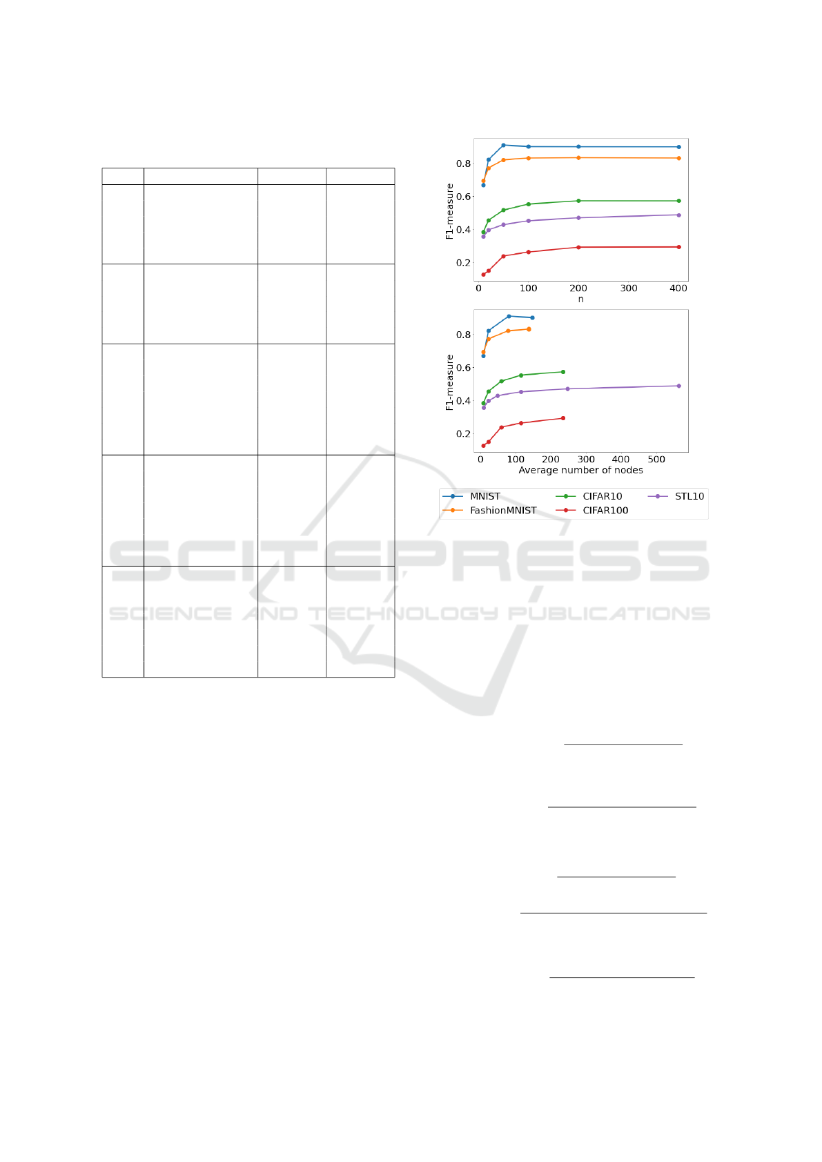
Table 2: Test accuracy and macro F1-measure in % for each

feature-set and dataset.

DS Feature Acc. F1

MNIST

Avg. color 60.8±1.4 59.5±1.5

Centroid 89.2±0.4 89.1±0.4

Std. dev. color 90.3±0.3 90.2±0.3

Std. dev. centroid 91.2±0.3 91.2±0.3

Num. of pixels 91.0±0.6 90.9±0.6

Fashion-

MNIST

Avg. color 61.4±1.0 61.2±1.4

Centroid 78.9±0.5 78.6±0.6

Std. dev. color 80.9±0.3 80.6±0.3

Std. dev. centroid 81.7±0.4 81.4±0.4

Num. of pixels 81.9±0.4 81.8±0.4

CIFAR10

Avg. color 41.2±0.9 40.7±0.8

Centroid 50.0±0.6 49.5±0.5

Std. dev. color 54.9±0.2 54.5±0.3

Std. dev. centroid 55.0±0.6 54.6±0.6

Num. of pixels 55.6±0.3 55.2±0.4

Avg. HSV 55.4±0.4 55.0±0.6

Std. dev. HSV 55.4±0.5 54.9±0.5

CIFAR100

Avg. color 16.9±0.4 15.1±0.5

Centroid 22.1±0.5 20.6±0.6

Std. dev. color 27.7±0.6 26.3±0.8

Std. dev. centroid 27.7±1.1 26.4±1.3

Num. of pixels 27.7±1.1 26.4±1.3

Avg. HSV 28.1±0.9 26.8±1.0

Std. dev. HSV 28.2±1.2 27.2±1.1

STL10

Avg. color 35.6±0.3 34.6±0.5

Centroid 38.6±0.5 37.4±0.3

Std. dev. color 43.5±2.0 42.9±1.6

Std. dev. centroid 44.4±0.6 43.5±0.8

Num. of pixels 44.7±1.0 44.0±1.0

Avg. HSV 46.8±0.5 46.5±0.3

Std. dev. HSV 47.1±0.7 46.4±0.8

knowledge – were chosen for this experiment:

• Region adjacency graphs (RAGs);

• K-Nearest Neighbors with spatial distance (KNN-

Spatial);

• K-Nearest Neighbors with combined spatial and

color distances (KNN-Combined).

In the region adjacency graphs, there is an edge

between two nodes if they correspond to directly ad-

jacent superpixels. That is, there is at least one pair

of pixels i and j, with coordinates (x

, y

) and (x

, y

each one belonging to each superpixel, that satisfy the

following condition:

− x

| + |y

− y

| = 1 (1)

The KNN-Spatial and KNN-Combined methods

attribute edges between each node and its k nearest

neighbors, not including the node itself. The differ-

ence between the two lies in the distance function:

Figure 4: Test F1-measure with macro average for, from

top to bottom, the value given as the desired number of

superpixels n, and the actual average number of superpix-

els/nodes produced by the SLICO algorithm.

KNN-Spatial compares two superpixels’ geometric

centroids while KNN-Combined combines the spatial

distance with the distance between average color val-

ues.

For two superpixels s

and s

, with geometric cen-

troids (x

, y

) and (x

, y

), and average color values

, g

, b

) and (r

, g

, b

) for RGB color datasets and

and l

for greyscale datasets, the spatial distance be-

tween s

and s

is given by:

spatial

, s

) =

− x

)

+ (y

− y

)

(2)

The combined color and spatial distance is deﬁned

as, for color datasets:

combined

, s

) =

′

spatial

, s

) + d

′

color

, s

) (3)

Where d

′

spatial

, s

) and d

′

color

, s

) are:

′

spatial

, s

) =

− x

)

+ (y

− y

)

(4)

′

color

, s

) =

− r

)

+ (g

− g

)

+ (b

− b

)

(5)

As for greyscale datasets, the combined color and spa-

tial distance is given by:

combined

, s

) =

′

spatial

, s

) + d

′

grey

, s

) (6)

ICEIS 2024 - 26th International Conference on Enterprise Information Systems

442

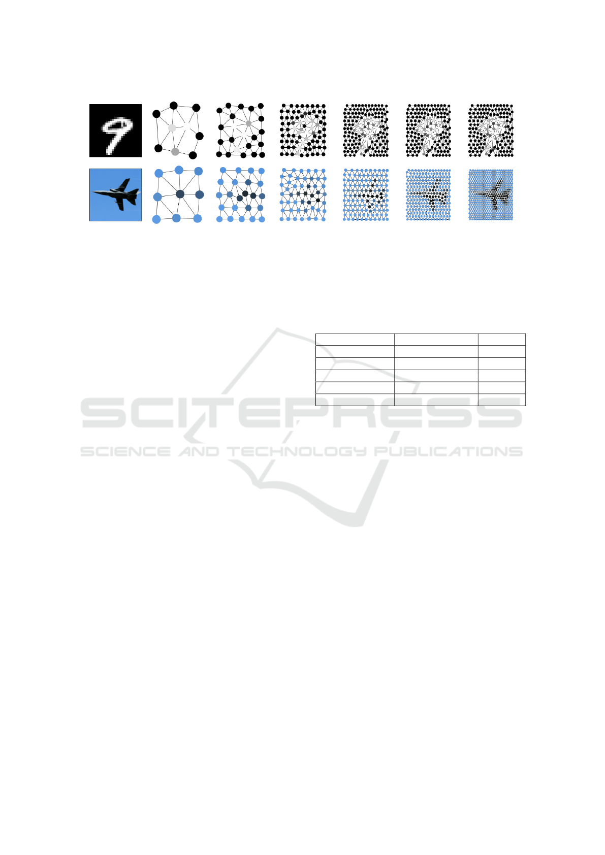
Figure 5: Examples of an original image and the RAGs generated for, from top to bottom, MNIST and STL-10 datasets. The

graphs were built using SLICO and n set to, from left to right, 10, 20, 50, 100, 200, and 400.

With d

′

grey

, s

) deﬁned as:

′

grey

= (l

− l

)

(7)

In this experiment, we used the following values

for the parameter k – that determines the node degree

– in the KNN-Spatial and KNN-Combined methods:

1, 2, 4, 8, and 16. It is important to note that self-

loops are always added in the training process and

that the node itself is not considered when comput-

ing its distances from the nodes in the graph. Figure

7 shows examples of graphs produced with the differ-

ent methods and parameter valuations, omitting said

self-loops.

We used as node features average color, centroid,

standard deviation of color, and standard deviation of

centroid. The segmentation method used was SLICO

with a ﬁxed desired number of nodes of 75.

Our results, as seen in Fig. 6, notably show

that performance tends to decrease as we increase

k, with most datasets. In general, the best perfor-

mance is achieved when k = 1, for both KNN-Spatial

and KNN-Combined. An exception to this pattern

is the MNIST dataset, whose best performance was

achieved when k = 2 for KNN-Combined, and when

k = 4 for KNN-Spatial. That suggests that the GCN

layers in the selected model are most helpful when the

information only ﬂows through uniform regions. As

we can see in Fig. 7, in the STL-10 1NN-Combined

graph, most of the airplane in the original image is

connected, while also being almost completely dis-

connected from the background sky.

That suggestion is corroborated by the tendency

of the KNN-Combined method to outperform both

KNN-Spatial and RAG (again, with the exception of

MNIST, in which the best results are achieved with

RAGs and then KNN-Spatial). As can be seen in Fig.

7, the KNN-Combined method tends to be more suc-

cessful in discriminating similar regions.

Since in RAGs, each node can have a variable

number of neighbors, in Table 3 we present the av-

erage degree of each node and the standard deviation

for RAGs generated for representing images in each

dataset. In general, the average degree is close to 5 in

all datasets.

Table 3: RAG’s average node degree and standard deviation

of node degree for each dataset.

Dataset Avg. node degree Std. dev.

MNIST 5.0 0.079

Fashion-MNIST 5.0 0.087

CIFAR-10 5.3 0.016

CIFAR-100 5.3 0.02

STL-10 5.1 0.062

3.5 Evaluating the Combination of Best

Parameters

In the previous experiments, we evaluated how the

different choices involved in the graph-building pro-

cess impact the performance of our GCN model re-

garding three dimensions: node features, number of

nodes, and method for building edges. However, in

each experiment, we tested different alternatives for

a given dimension and kept the other two dimensions

ﬁxed. In this experiment, for each dataset, we identi-

ﬁed the choice that resulted in the best performance

for each of the 3 dimensions. After that, we built

graphs for representing images in each dataset, by

combining the best choices identiﬁed in the previ-

ous experiments. Table 4 presents the best choices

for each dimension and each dataset, along with the

performances achieved by the model taking as input

graphs built by combining such choices. In Table 4,

F1 corresponds to the feature-set {average color, stan-

dard deviation of color, centroid, standard deviation

from centroids, number of pixels} and F2 corresponds

to F1 ∪ {average HSV color, standard deviation of

HSV color}.

From the results in Table 4 we can notice that the

best combination achieved the best performance in

Graph Convolutional Networks for Image Classiﬁcation: Comparing Approaches for Building Graphs from Images

443

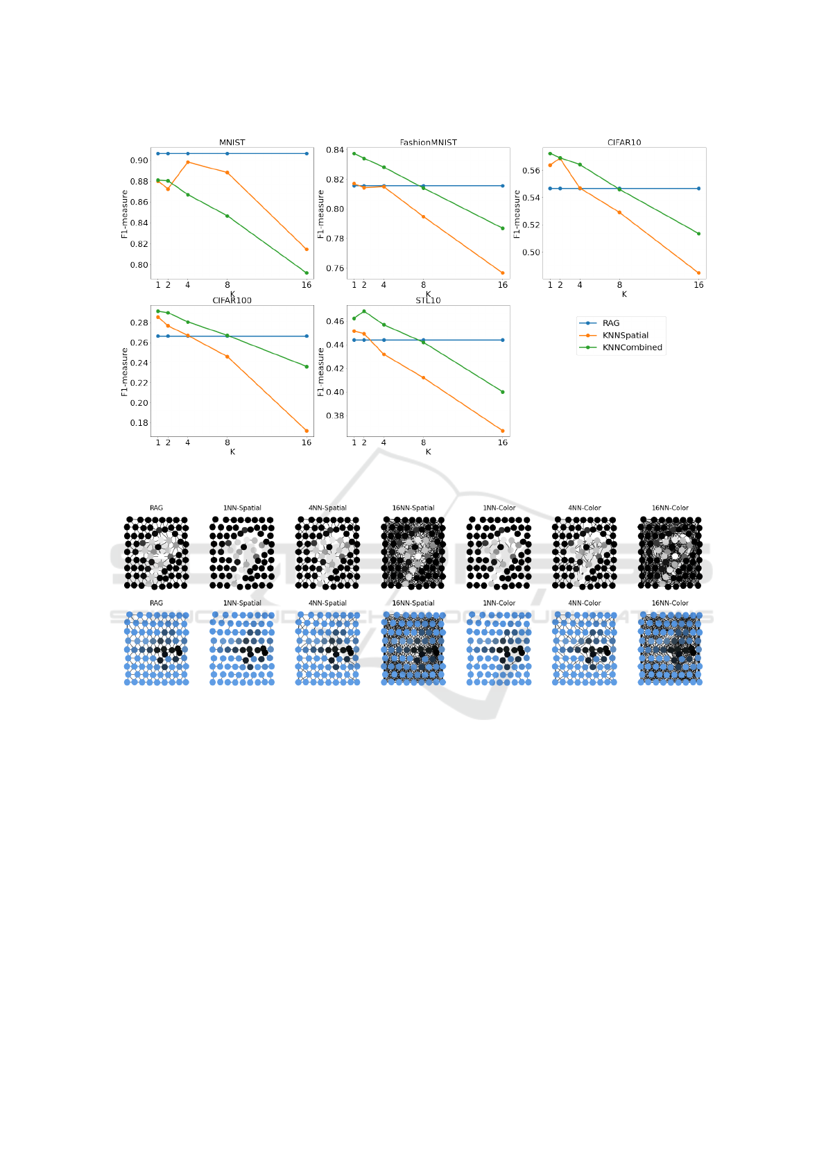
Figure 6: Macro F1-measure in the test set for each dataset with respect to the k parameter of KNN-Spatial and KNN-

Combined methods, with RAG’s performance shown ﬁxed for visualization.

Figure 7: Examples of selected graphs produced in the experiment from the same original images shown in Fig. 5 for MNIST

and STL-10 datasets, each with approximately 75 nodes.

comparison with the best results achieved in the previ-

ous experiments. The exception is MNIST, for which

the best result was achieved with the same feature-set

and edge-building method but with 75 nodes in the

feature-ser assessment experiment with 91.7±0.2 F1-

measure and 91.8±0.2 accuracy.

4 CONCLUSIONS

In this paper, we have systematically analyzed the im-

pacts on the performance of a GCN model for image

classiﬁcation depending on how we build graphs for

representing images. We evaluated three dimensions

of the graph-building process: node feature selection,

degree of segmentation (number of nodes), and the

approaches for building edges.

We have found that, for the selected datasets, in-

creasing the degree of segmentation and, therefore,

the number of nodes in the graph has a positive im-

pact on the model’s performance. This is expected,

since, as the number of nodes increases, more details

of the original image are represented. However, the

gain in performance follows approximately a loga-

rithmic curve, decreasing as the number of nodes ap-

proaches the total number of pixels. Thus, it is im-

portant to consider this information when using such

approaches, since the memory requirements for stor-

ing graph information grow linearly with the number

of nodes.

The selection of more descriptive features tends to

have a positive effect, compensating for the loss of in-

ICEIS 2024 - 26th International Conference on Enterprise Information Systems

444

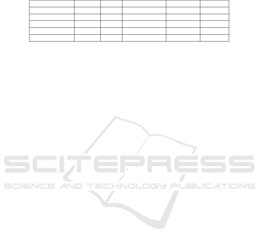
Table 4: For each dataset and graph-building choice, test F1-measure with macro average and accuracy for the combination

of the best-performing choices.

Dataset Features Nodes Graph type F1-measure Accuracy

MNIST F1 50 RAG 91.2±0.4 91.3±0.4

Fashion-MNIST F1 200 1NN-Combined 84.0±0.4 84.2±0.4

CIFAR-10 F2 400 1NN-Combined 58.3±0.7 58.5±0.6

CIFAR-100 F2 200 1NN-Combined 30.9±1.1 32.2±0.8

STL-10 F2 400 2NN-Combined 51.8±0.6 52.1±0.4

formation in the segmentation process. The most sig-

niﬁcant increase in performance is seen when adding

spatial information (i.e.: each superpixel’s geomet-

ric centroid) to the color information. However, we

note that the often-suggested pixel-density feature has

been detrimental to the performance in some of the

selected datasets.

By comparing the approaches for building edges,

we have found that, in most cases, increasing the size

of each node’s neighborhood results in a decrease in

performance. The best results were achieved when

neighborhoods were restricted to similar regions.

Grounds for future work include expanding the

analysis to other GNN architectures such as Graph

Attention Networks ((Veli

ckovi

c et al., 2018)), ex-

ploring the effects of the levels of irregularity of the

image segments (as parameterized by the smoothness

factor in the basic SLIC algorithm), as well as explor-

ing the effects of other methods of image segmenta-

tion.

REFERENCES

Achanta, R., Shaji, A., Smith, K., Lucchi, A., Fua, P., and

usstrunk, S. (2012). SLIC Superpixels Compared to

State-of-the-Art Superpixel Methods. IEEE Transac-

tions on Pattern Analysis and Machine Intelligence,

34(11):2274–2282. Conference Name: IEEE Trans-

actions on Pattern Analysis and Machine Intelligence.

Achanta, R. and Susstrunk, S. (2017). Superpixels

and Polygons Using Simple Non-Iterative Clustering.

pages 4651–4660.

Avelar, P. H. C., Tavares, A. R., da Silveira, T. L. T., Jung,

C. R., and Lamb, L. C. (2020a). Superpixel Im-

age Classiﬁcation with Graph Attention Networks. In

2020 33rd SIBGRAPI Conference on Graphics, Pat-

terns and Images (SIBGRAPI), pages 203–209. ISSN:

2377-5416.

Avelar, P. H. C., Tavares, A. R., da Silveira, T. L. T., Jung,

C. R., and Lamb, L. C. (2020b). Superpixel Im-

age Classiﬁcation with Graph Attention Networks. In

2020 33rd SIBGRAPI Conference on Graphics, Pat-

terns and Images (SIBGRAPI), pages 203–209, Re-

cife/Porto de Galinhas, Brazil. IEEE.

Bessadok, A., Mahjoub, M. A., and Rekik, I. (2022). Graph

neural networks in network neuroscience. IEEE

Transactions on Pattern Analysis and Machine Intel-

ligence, 45(5):5833–5848.

Chen, B., Li, J., Lu, G., Yu, H., and Zhang, D. (2020). Label

co-occurrence learning with graph convolutional net-

works for multi-label chest x-ray image classiﬁcation.

IEEE journal of biomedical and health informatics,

24(8):2292–2302.

Chen, C., Wu, Y., Dai, Q., Zhou, H.-Y., Xu, M., Yang,

S., Han, X., and Yu, Y. (2022). A survey on graph

neural networks and graph transformers in computer

vision: A task-oriented perspective. arXiv preprint

arXiv:2209.13232.

Coates, A., Lee, H., and Ng, A. Y. An Analysis of Single-

Layer Networks in Unsupervised Feature Learning.

Defferrard, M., Bresson, X., and Vandergheynst, P. (2016).

Convolutional Neural Networks on Graphs with Fast

Localized Spectral Filtering. In Advances in Neural

Information Processing Systems, volume 29. Curran

Associates, Inc.

Du, H., Yao, M. M.-S., Liu, S., Chen, L., Chan, W. P., and

Feng, M. (2023). Automatic calciﬁcation morphology

and distribution classiﬁcation for breast mammograms

with multi-task graph convolutional neural network.

IEEE Journal of Biomedical and Health Informatics.

Errica, F., Podda, M., Bacciu, D., and Micheli, A. (2022). A

Fair Comparison of Graph Neural Networks for Graph

Classiﬁcation. arXiv:1912.09893 [cs, stat].

Hong, D., Gao, L., Yao, J., Zhang, B., Plaza, A., and

Chanussot, J. (2020). Graph convolutional net-

works for hyperspectral image classiﬁcation. IEEE

Transactions on Geoscience and Remote Sensing,

59(7):5966–5978.

Kipf, T. N. and Welling, M. (2017). Semi-Supervised

Classiﬁcation with Graph Convolutional Networks.

arXiv:1609.02907 [cs, stat].

Krizhevsky, A. Learning Multiple Layers of Features from

Tiny Images.

Lecun, Y., Bottou, L., Bengio, Y., and Haffner, P. (1998).

Gradient-based learning applied to document recog-

nition. Proceedings of the IEEE, 86(11):2278–2324.

Conference Name: Proceedings of the IEEE.

Linh, L. V. and Youn, C.-H. (2021). Dynamic Graph

Neural Network for Super-Pixel Image Classiﬁca-

tion. In 2021 International Conference on Infor-

mation and Communication Technology Convergence

(ICTC), pages 1095–1099. ISSN: 2162-1233.

Long, J., yan, Z., and chen, H. (2021). A Graph Neural

Network for superpixel image classiﬁcation. Journal

of Physics: Conference Series, 1871(1):012071.

Graph Convolutional Networks for Image Classiﬁcation: Comparing Approaches for Building Graphs from Images

445

Monti, F., Boscaini, D., Masci, J., Rodol

a, E., Svoboda, J.,

and Bronstein, M. M. (2016). Geometric deep learn-

ing on graphs and manifolds using mixture model

CNNs. arXiv:1611.08402 [cs] version: 3.

Reiser, P., Neubert, M., Eberhard, A., Torresi, L., Zhou,

C., Shao, C., Metni, H., van Hoesel, C., Schopmans,

H., Sommer, T., et al. (2022). Graph neural networks

for materials science and chemistry. Communications

Materials, 3(1):93.

Scarselli, F., Gori, M., Tsoi, A. C., Hagenbuchner, M.,

and Monfardini, G. (2009). The Graph Neural Net-

work Model. IEEE Transactions on Neural Networks,

20(1):61–80. Conference Name: IEEE Transactions

on Neural Networks.

Shchur, O., Mumme, M., Bojchevski, A., and G

unnemann,

S. (2019). Pitfalls of Graph Neural Network Evalua-

tion. arXiv:1811.05868 [cs, stat].

Shlomi, J., Battaglia, P., and Vlimant, J.-R. (2020). Graph

neural networks in particle physics. Machine Learn-

ing: Science and Technology, 2(2):021001.

Stutz, D., Hermans, A., and Leibe, B. (2018). Superpixels:

An evaluation of the state-of-the-art. Computer Vision

and Image Understanding, 166:1–27.

Tang, T., Chen, X., Wu, Y., Sun, S., and Yu, M. (2022). Im-

age classiﬁcation based on deep graph convolutional

networks. In 2022 IEEE 9th International Conference

on Data Science and Advanced Analytics (DSAA),

pages 1–6. IEEE.

Todescato, M. V., Garcia, L. F., Balreira, D. G., and Car-

bonera, J. L. (2024). Multiscale patch-based feature

graphs for image classiﬁcation. Expert Systems with

Applications, 235:121116.

Van den Bergh, M., Boix, X., Roig, G., and Van Gool, L.

(2015). SEEDS: Superpixels Extracted Via Energy-

Driven Sampling. International Journal of Computer

Vision, 111(3):298–314.

Veli

ckovi

c, P., Cucurull, G., Casanova, A., Romero, A., Li

P., and Bengio, Y. (2018). Graph Attention Networks.

arXiv:1710.10903 [cs, stat].

Wu, L., Chen, Y., Shen, K., Guo, X., Gao, H., Li, S., Pei,

J., Long, B., et al. (2023). Graph neural networks for

natural language processing: A survey. Foundations

and Trends® in Machine Learning, 16(2):119–328.

Wu, Z., Pan, S., Chen, F., Long, G., Zhang, C., and Philip,

S. Y. (2020). A comprehensive survey on graph neural

networks. IEEE transactions on neural networks and

learning systems, 32(1):4–24.

Xiao, H., Rasul, K., and Vollgraf, R. (2017). Fashion-

MNIST: a Novel Image Dataset for Benchmarking

Machine Learning Algorithms. arXiv:1708.07747 [cs,

stat].

Xu, K., Hu, W., Leskovec, J., and Jegelka, S.

(2019). How Powerful are Graph Neural Networks?

arXiv:1810.00826 [cs, stat].

Yao, J., Boben, M., Fidler, S., and Urtasun, R. (2015). Real-

Time Coarse-to-Fine Topologically Preserving Seg-

mentation. pages 2947–2955.

Yassine, B., Taylor, P., and Story, A. (2018). Fully auto-

mated lung segmentation from chest radiographs us-

ing slico superpixels. Analog Integrated Circuits and

Signal Processing, 95(3):423–428.

Zhang, W., Joseph, J., Yin, Y., Xie, L., Furuhata, T., Ya-

makawa, S., Shimada, K., and Kara, L. B. (2023).

Component segmentation of engineering drawings us-

ing graph convolutional networks. Computers in In-

dustry, 147:103885.

Zhang, X.-M., Liang, L., Liu, L., and Tang, M.-J. (2021).

Graph neural networks and their current applications

in bioinformatics. Frontiers in genetics, 12:690049.

ICEIS 2024 - 26th International Conference on Enterprise Information Systems

446