
State-Aware Application Placement in Mobile Edge Clouds
Chanh Nguyen
a
, Cristian Klein
b
and Erik Elmroth
c
Department of Computing Science, Ume
˚
a University, Sweden
Keywords:
Mobile Edge Clouds, Application Placement, Service Orchestration, Optimization.
Abstract:
Placing applications within Mobile Edge Clouds (MEC) poses challenges due to dynamic user mobility. Main-
taining optimal Quality of Service may require frequent application migration in response to changing user
locations, potentially leading to bandwidth wastage. This paper addresses application placement challenges
in MEC environments by developing a comprehensive model covering workloads, applications, and MEC
infrastructures. Following this, various costs associated with application operation, including resource utiliza-
tion, migration overhead, and potential service quality degradation, are systematically formulated. An online
application placement algorithm, App EDC Match, inspired by the Gale-Shapley matching algorithm, is in-
troduced to optimize application placement considering these cost factors. Through experiments that employ
real mobility traces to simulate workload dynamics, the results demonstrate that the proposed algorithm effi-
ciently determines near-optimal application placements within Edge Data Centers. It achieves total operating
costs within a narrow margin of 8% higher than the approximate global optimum attained by the offline pre-
cognition algorithm, which assumes access to future user locations. Additionally, the proposed placement
algorithm effectively mitigates resource scarcity in MEC.
1 INTRODUCTION
The growth of mobile technology, coupled with the
rollout of 5G networks, paves the way for a new era
of applications characterized by stringent demands
for minimal jitter, low latency, and extensive band-
width. As an example, real-time gaming applications
necessitate response times of mere milliseconds to
forestall substantial Quality of Service (QoS) degra-
dation (Pantel and Wolf, 2002). Likewise, virtual
reality applications employing head-tracked systems
mandate latencies below 16 ms to maintain percep-
tual stability, preserving the illusion of reality (Ellis
et al., 2004).
In recent years, there has been a significant shift
away from conventional centralized cloud comput-
ing data centers towards the adoption of a dis-
tributed computing infrastructure known as Mobile
Edge Clouds (MECs). MECs are designed to de-
centralize computing and storage resources to the
network edge, specifically within Edge Data Cen-
ters (EDCs) located in close proximity to end-users.
These EDCs are often strategically placed, such as
a
https://orcid.org/0000-0002-9156-3364
b
https://orcid.org/0000-0003-0106-3049
c
https://orcid.org/0000-0002-2633-6798
being colocated with central office locations (Kavak
et al., 2015). Recent research efforts (Mehta et al.,
2016; Tong et al., 2016) have introduced the con-
cept of hierarchical MECs, incorporating heteroge-
neous costs and capacities. In this hierarchical struc-
ture, data centers (DCs) are organized into different
layers. DCs in higher layers offer greater compu-
tational capacities at lower cost but are situated far-
ther from end-users, resulting in increased latency and
bandwidth expenses. MECs offer exceptional flexi-
bility, allowing for the placement of applications that
align with their specific requirements. This versatility
strikes a balance between cost-effective computation
and proximity to end-users. In fact, many algorithms
have been proposed for placing stateless applications
on MECs, including dynamic placement algorithms
for efficiently dealing with user mobility (Li et al.,
2022; Shang et al., 2022; Apat et al., 2023; Nguyen
et al., 2019). Nonetheless, a significant number of en-
visioned MEC applications exhibit stateful character-
istics. Take, for instance, augmented reality applica-
tions, which entail the storage of generated meshes,
world data, textures, and more. Utilizing stateless
placement algorithms for such stateful applications
entails the risk of incurring unnecessary costs, primar-
ily attributed to the bandwidth needed to migrate user
Nguyen, C., Klein, C. and Elmroth, E.
State-Aware Application Placement in Mobile Edge Clouds.
DOI: 10.5220/0012326300003711
Paper published under CC license (CC BY-NC-ND 4.0)
In Proceedings of the 14th International Conference on Cloud Computing and Services Science (CLOSER 2024), pages 117-128
ISBN: 978-989-758-701-6; ISSN: 2184-5042
Proceedings Copyright © 2024 by SCITEPRESS – Science and Technology Publications, Lda.
117

state from one EDC to another.
In this paper, we tackle the challenge of placing
stateful applications in an MEC environment. Our ap-
proach begins with a comprehensive modeling of the
various costs associated with hosting stateful applica-
tions on MECs. These costs encompass the resource
cost, which includes both computing and application
bandwidth expenses, as well as the QoS degradation
cost and migration costs. Subsequently, we introduce
an online state-aware application placement strategy,
denoted as App EDC Match, inspired by the well-
known Gale-Shapley matching algorithm (Gale and
Shapley, 1962). The primary objective of the pro-
posed strategy is to discover placement solutions that
match applications with EDCs, resulting in the lowest
resource cost and bandwidth consumption across the
physical network links.
We conducted a comprehensive evaluation of the
proposed algorithms within an MEC topology encom-
passing EDCs distributed throughout the San Fran-
cisco area. To simulate user mobility patterns, we em-
ployed real mobility traces derived from taxi move-
ment data in San Francisco. Additionally, we mod-
eled user transitions between applications using a
Markov model. The evaluation compared the total op-
erating costs generated by the App EDC Match algo-
rithm against those produced by a precognition place-
ment algorithm, which possesses knowledge of future
user locations. Furthermore, we conducted extensive
experimental comparisons of the proposed placement
algorithm’s performance and behavior across differ-
ent application types, including compute-intensive
and bandwidth-intensive applications.
The contributions of this paper are three-fold:
• A comprehensive cost model is provided for host-
ing stateful applications on MECs (see Section 2).
• An efficient online state-aware placement strategy
for distributing applications among EDCs with
the goal of minimizing the overall operating costs
(see Section 3).
• Extensive experiments to evaluate the perfor-
mance of the proposed placement strategy (see
Section 5).
The experimental results show the efficiency of
the proposed online placement algorithm for optimiz-
ing application placements among EDCs. It achieves
a total operational cost only 8% higher than the ap-
proximate global optimum determined by the pre-
cognition offline algorithm. Furthermore, the pro-
posed algorithm effectively addresses workload bal-
ancing within MECs, mitigating resource scarcity
challenges.
2 PROBLEM DEFINITION
In this section, we first describe models for each com-
ponent considered in the application placement prob-
lem, namely the MEC infrastructure, applications,
user mobility, workload and cost model. Based on
these models, we then formulate a formal statement
of the problem to be solved.
2.1 Mobile Edge Clouds
MECs with a hierarchy of geo-distributed EDCs have
proven to be efficient infrastructures for meeting en-
visioned MEC workloads (Tong et al., 2016; Bar-
tolomeo et al., 2023; Yang et al., 2018; Wang et al.,
2017). We therefore focus on a MEC with EDCs
organized into a hierarchical topology in this work
(see Figure 1).
We model a MEC as a set of N EDCs geograph-
ically distributed within an area, denoted E = {i|i =
1,2,...,N}. Each EDC is identified by a geographic
location loc
i
and a layer that e
i
belongs to. In layer
1, every EDC e
i
is collocated with a cellular base
station or a WiFi access point, from which the end-
users send requests to an application hosted by the
MEC. Each EDC is equipped with a certain number
of servers that provide a pool of virtualized comput-
ing resources. EDCs in higher layers feature greater
computing capacities. We use C
i
to denote the com-
puting capacity of e
i
.
The interconnection between the EDCs is repre-
sented by the following network model. We denote
the set of all physical network links in the MEC as
L = { j| j = 1,2,...,M}. Each link l
j
connects e
i
with
its closest ancestor and is characterized by its network
delay d
j
and a maximum bandwidth – also known as
the bandwidth capacity – denoted B
j
. Thus, it is worth
noting that M = N − 1. Any pair of EDCs can com-
municate by following the shortest network path. Let
P
i,i
′
⊆ L be the set of all physical network links on
the shortest path between two EDCs e
i
, e
i
′
. Here, it is
worth noting that total bandwidth consumed on a par-
ticular physical network link l
j
is equal to the sum of
the bandwidth consumed on all paths P
i,i
′
containing
l
j
.
2.2 Application
Let A = {p|p = 1,2,..,P} be the set of applications
hosted in the MEC. An application p is characterized
by the following parameters:
• Compute ξ
c
p
describes the amount of computa-
tional resource units required by p to serve an end-
user. The unit is CPU × seconds/user.
CLOSER 2024 - 14th International Conference on Cloud Computing and Services Science
118

e
9
e
8
e
1
e
2
e
4
e
5
e
7
Layer 1
Layer 2
Layer 3
l
1
l
2
l
3
l
4
l
5
l
6
e
3
e
6
l7 l8
Figure 1: Our model of an MEC, showing the organization
of EDCs into various layers and physical network linking
the EDCs.
• Bandwidth ξ
b
p
describes the amount of network
bandwidth required by p to serve an end-user. The
unit is KB/user.
• State ξ
s
p
describes the amount of state stored by
p for each served end-user. This is the amount
of network bandwidth required to transfer the ap-
plication from one EDC to another. The unit is
KB/user.
We use compute-bandwidth-usage-ratio per applica-
tion request (CPU-h/GB), denoted as A
cl
(Mehta
et al., 2016), to determine whether a specific appli-
cation is compute-intensive or bandwidth-intensive.
A
cl
takes values in the range [0.01,10]. To guaran-
tee the target QoS, the system must allocate resources
(both compute and bandwidth) that can handle the to-
tal workload generated by users.
2.3 User and Workload
We consider a set of users U = {k|k = 1,2,...,K} that
dynamically move around in the area covered by the
MEC. In time slot t, user k connects wirelessly to the
physically closest EDC, called the connecting EDC.
The access delay, i.e., the delay due to the wireless
network between k and the connecting EDC i is de-
noted as d
k,t
.
In each time slot t, user k connect to application
p ∈ A that is specified in λ
k,t
. After each time slot,
user k may continue using the same application or
change to a different application.
To serve the user, the placement algorithm must
allocate capacity to the application in a serving EDC.
Depending on the placement algorithm’s decision,
the serving EDC may or may not coincide with the
connecting EDC. Let s
k,t,i
denote the decision about
whether or not the requested application p of user k is
hosted on i at time slot t. Formally:
s
k,t,i
=
(
1, if p is hosted in EDC i for user k
0, otherwise
(1)
and
∑
i
s
k,t,i
= 1
(2)
Let tb
j,t
be the total bandwidth (i.e. the bandwidth
allocated for serving applications plus the bandwidth
needed to migrate applications) allocated from link j
in time slot t. This gives us the expression:
tb
j,t
= ξ
b
j,t
+ ξ
s
j,t
(3)
whereas, ξ
b
j,t
is total bandwidth allocated on net-
work link j for serving applications in time slot t, and
ξ
s
j,t
is total bandwidth allocated on network link j for
migrating applications in time slot t.
2.4 Operating Cost
To serve the end-users, the system responsible for
placing applications hosted in MECs must take var-
ious costs into consideration:
• The Resource Cost:
This cost refers to the compute and bandwidth
cost, which abstract all the regular costs due to
hardware, service maintenance, energy consump-
tion, and so on. While real cloud computing sys-
tems employ intricate unit pricing functions, con-
sidering factors like supply and demand, resource
utilization, instance types, and pricing tiers, our
modeling approach simplifies this by assuming
an inverse proportionality between the current ca-
pacities of compute resource at EDC i and net-
work link j with their respective unit prices. This
simplification adheres to micro-economic prin-
ciples, particularly the law of supply and de-
mand (Moore, 1925), and acknowledges the influ-
ence of economy-of-scale effects on energy and
maintenance costs. It is worth noting that the
resource unit price function (as defined in equa-
tion 4 below) can be customized to align with
stakeholder definitions and specific scenarios.
Let g
∗
(.) be the function that determines the re-
source unit price:
g
∗
(x
t
) = (u
max
− u
min
) × x
t
+ u
min
(4)
Here,
x
t
=
∑
k
s
k,t−1,i
×ξ
c
λ
k,t−1
C
i
,for the compute resource
tb
j,t−1
B
j
, for the bandwidth resource
(5)
and u
min
,u
max
are the minimum and maximum re-
source unit price, which are predefined differently
for each EDC i and network link j.
The resource cost Cost
res
is then calculated as be-
low:
State-Aware Application Placement in Mobile Edge Clouds
119

Cost
res
=
∑
t
∑
i
∑
k
s
k,t,i
×
g
i
× ξ
c
λ
k,t
+
∑
j∈P
i,loc
u
k
,t
g
j
× ξ
b
λ
k,t
(6)
Here, P
loc
k,t
,i
is the network path as defined in Sec-
tion 2.1.
The total bandwidth allocated on a particular
physical network link j for serving applications
is equal to the sum of the bandwidth consumed
on paths P
loc
k,t
,i
go through j, which is decided by
s
k,t,i
:
ξ
b
j,t
=
∑
k
∑
j∈P
loc
k,t
,i
s
k,t,i
× ξ
b
λ
k,t
(7)
• The Migration Cost: This cost is associated with
migrations, i.e. the transfer of a user’s application
p hosted on EDC i at time t − 1 to another EDC
i
′
in time slot t. It is related to the size of the ap-
plication’s state data (or service profile) for each
user. Transferring such data across EDCs requires
bandwidth from the inter-EDC-network connect-
ing i and i
′
.
We define the migration flag as MF
k,t,i,i
′
, which
takes a value of 1 if and only if user k requests
the same application in successive time slots (i.e.,
λ
k,t
= λ
k,t−1
), and that application is placed on
different EDCs in those time slots (i.e., ⟨s
k,t
·
s
k,t−1
⟩ = 0):
MF
k,t,i,i
′
=
1, λ
k,t
= λ
k,t−1
,
and s
k,i
′
,t
= 1
and s
k,i,t−1
= 1
0, otherwise
(8)
Here, i is the source EDC and i
′
is the destination
EDC of the migration.
Then, the total migration cost is calculated as:
Cost
mig
=
∑
t
∑
k
∑
i
∑
i
′
(MF
k,t,i,i
′
×
∑
j∈P
i,i
′
g
j
× ξ
s
λ
k,t
)
(9)
Here, the total bandwidth allocated on a network
link l
j
for application migrations is equal to the
sum of the bandwidth allocated to migrate appli-
cations on paths P
i,i
′
going through l
j
:
ξ
s
j,t
=
∑
k
∑
i
∑
i
′
MF
k,t,i,i
′
×
∑
j∈P
i,i
′
ξ
s
λ
k,t
(10)
• The Service Quality Degradation Cost: This
cost stems from delays due to three factors: i) the
start-up time of new virtual resources to host new
applications requested by users; ii) the wireless
network delay between user k and the connected
EDC e
i
; and iii) the delay due to data transmission
between network link l
j
(including data transmis-
sion due to an application’s state migration, if
any).
Given ξ
c
λ
k,t−1
and ξ
c
λ
k,t
, we calculate the increment
of the resource allocation for EDC e
i
between two
time slots t and t − 1 as below:
δ
t,i
= max
(
∑
k
s
k,t,i
× ξ
c
λ
k,t
− s
k,t−1,i
× ξ
c
λ
k,t−1
,
0
)
(11)
Denoting the average start-up time for a new vir-
tual resource as st, we assume the new virtual re-
sources are invoked in parallel at each EDC e
i
in
each time slot t. The start-up time of the new
added virtual resources, d
st,t
, is thus given by the
following expression:
d
st,t
=
(
st, for δ
t,i
> 0
0, for δ
t,i
= 0
(12)
To model the relationship between the network la-
tency and the injection bandwidth for each phys-
ical link l
j
, we treat the relative latency as a
function of the offered traffic for a simple net-
work. As shown previously (Moudi and Othman,
2020; Dally and Towles, 2004), the network la-
tency in an interconnection network rises to infin-
ity as throughput approaches saturation. In such
cases, the relationship is well described by an ex-
ponential distribution. It is worth noting that in
our model, we constrain the total bandwidth allo-
cation on each link l
j
at time t to the link’s max-
imum bandwidth. Consequently, we do not ac-
count for potential waiting times, such as queuing
latency, that may be present in an actual network.
We model the network delay at link l
j
using an
exponential distribution:
delay
j,t
=
e
tb
j,t
B
j
1 −
tb
j,t
B
j
+ d
j
(13)
Let cc
qos
be the unit price of the service qual-
ity downgrade due to delay. The service quality
degradation cost, Cost
qos
, can then be calculated
CLOSER 2024 - 14th International Conference on Cloud Computing and Services Science
120

as follows:
Cost
qos
= cc
qos
×
∑
t
d
st,t
+
∑
k
d
k,t
+
∑
l
j
delay
l
j
,t
(14)
2.5 Cost Optimization Formulation
Having describing different costs of placing applica-
tions on MECs to serve end-users respecting to QoS.
The total cost is the sum of all the aforementioned
costs, i.e., Cost
res
+ Cost
mig
+ Cost
qos
. The applica-
tion placement optimization problem can be formal-
ized as:
minimize: P = Cost
res
+ Cost
mig
+ Cost
qos
(15)
subject to:
∑
k
ξ
c
λ
k,t
× s
k,i,t
≤ C
i
,∀i,t, (16)
tb
j,t
≤ B
j
,∀ j,t (17)
Here, constraints 16 and 17 ensure that the system’s
capacity limit is not exceeded (i.e. the load on each
EDC does not exceed its compute capacity; and the
traffic through each network link does not exceed its
maximum bandwidth).
In summary, in each time slot t ∈ T , the system
must decide s
k,t,i
, i.e., on which EDCs to place the
requested application p of user k. These decisions de-
termine the total compute resource allocation at each
EDC e
i
, and total bandwidth usage at each link l
j
.
The decision should be made so as to guarantee that
the aggregated operating cost over time window T is
minimized.
3 ONLINE APPLICATION
PLACEMENT ALGORITHM
In this section, we first present the mathematical
transformation to simplify the original placement
problem presented in Section 2. Subsequently, we
establish the NP-hardness of the placement prob-
lem, highlighting the impracticality of obtaining an
exact solution within polynomial time. In light of
these challenges, we introduce the App EDC Match
placement strategy, an online placement algorithm de-
signed to address the placement problem efficiently
within polynomial time.
3.1 Mathematical Transformation and
NP-Hardness Proof
It is undoubtedly true that in time slot t the place-
ment decisions made in previous time slots cannot be
changed. However, the placement of applications in
the preceding time slot t − 1 will impact the place-
ment decision at time t. Therefore, the original total
operation cost P from Equation (15) can be re-written
as follows (with T = [1, T ]):
P
t∈[1,T ]
= P
t∈[1,T −1]
+ P
t=T
(18)
Finding an optimal operating cost P
t∈[1,T ]
thus be-
comes a recursive process of finding an optimal oper-
ating cost P
t=T
based on the current system’s state,
and the assumption that the application placements
decided in the previous time slots t ≤ T − 1 are op-
timal. In each time slot t ∈ T , the total compute re-
source allocated at each EDC e
i
,
∑
k
ξ
c
k,t−1
× s
k,t−1,i
and the total bandwidth resource allocated at each net-
work link l
j
, tb
j,t−1
are known. These values together
with the users’ application requests and their loca-
tion during t are the inputs for the placement prob-
lem, P
t=T
. Therefore, the original placement prob-
lem transforms into an assignment problem: to which
EDC should each user’s requested applications be as-
signed so as to minimize the total operating cost at
every time slot t. This problem has been proven to be
NP-hard (Fisher et al., 1986).
Obtaining an optimal solution for the application
placement problem in polynomial time is considered
impossible unless P = NP. Consequently, our focus
shifts to the development of efficient algorithms ca-
pable of delivering near-optimal solutions for min-
imizing P
t=T
within a polynomial time frame. In
pursuit of this goal, we present the App EDC Match
placement strategy, an efficient heuristic algorithm in-
spired by the widely recognized Gale-Shapley match-
ing problem.
3.2 App EDC Match Placement
Strategy
In general, our problem of assigning requested appli-
cations to EDCs in each time slot t to minimize P
t=T
is analogous to the college admissions discussed by
Gale and Shapley (Gale and Shapley, 1962). In the
college admissions problem, each student proposes
to their most preferred available college, while col-
leges can only hold a limited number of proposals at
a time. Subsequently, a solution is derived to match
students with colleges based on their preferences and
constraints, with the goal of optimizing criteria such
as overall satisfaction or fairness. The set of n EDCs
State-Aware Application Placement in Mobile Edge Clouds
121

E can be compared to the set of n colleges, in which
each e
i
∈ E has a designated “quota” C
i
. Similarly,
the set of m requested applications, to be assigned to
the n EDCs, can be compared to the m applicants to
be assigned to the n colleges. Inspired by this parallel,
we introduce the App EDC Macth placement strategy
leveraging the Gale-Shapley algorithm as presented in
Algorithm 1.
The algorithm receives inputs that encompass the
application placement solution from time t − 1, com-
pute resource availability at each EDC, and band-
width availability at each network link up to time
t (line 1). Subsequently, the algorithm updates the
compute unit price and bandwidth unit price at each
EDC e
i
and network link l
j
respectively (line 2).
Moving forward, the algorithm proceeds to construct
the application preference matrix M
app
(n× m), where
each column p ranks EDCs in decreasing order of the
operating cost incurred when placing application p on
them (line 3). Similarly, the algorithm formulates an
EDC preference matrix M
edc
(m × n), where each col-
umn i ranks the requested applications in decreasing
order of the bandwidth consumption when placed on
EDC e
i
(line 4). This preference ensures that each ap-
plication is hosted on an EDC that minimizes network
congestion. Finally, it invokes the matching method
to perform the assignment, using the two matrices
above as inputs (line 5).
For n EDCs and m applications, the time com-
plexity of the App EDC Match placement strategy is
O(n × m).
1: Input: The application placement from t − 1,
Datacenters resource capacity up to t,
Network links bandwidth capacity up to t,
User locations u
k
and workload W = λ
k,t
at t
2: Update: compute unit price of each EDC i,
bandwidth unit price of each network link j
3: Calculate M
app
(n × m) – the application prefer-
ence matrix, in which each column p ranks EDCs
in the order of resulting lowest operating cost if
application p is placed on it
4: Calculate M
edc
(m × n) – the EDC preference
matrix, in which each column i rank applications
in the order of consuming least bandwidth
5: Matching (M
app
, M
edc
)
6: return s
k,i
, cost
Algorithm 1: App EDC Match placement strategy.
4 EXPERIMENTAL SETTING
This section presents our simulation-based evalua-
tion. First, we describe an MEC infrastructure with
EDCs distributed in a metropolitan area connected in
e1
e2
e3
e4
e5
e6
Figure 2: Distribution of 6 EDCs collocated with cellular
base stations in layer 1.
tree topology. Then, we describe the parameters of
simulated applications and end-users workload. Fi-
nally, we describe the implementation and setup of
our proposed placement algorithm, as well as the
baseline placement algorithm.
4.1 Infrastructure: an MEC Platform
We simulate a hierarchical MEC platform with EDCs
distributed over a metropolitan area, drawing on a pre-
viously reported MEC model (Mehta et al., 2016).
The capacities of EDCs in different layers and their
compute unit price (min, max) are presented in Ta-
ble 1 together with the capacities and prices of the net-
work links between subsequent layers. The physical
network links between layer 1 and layer 2 are mod-
eled as OC-3 (i.e., optical carrier level 3), while the
links between layer 2 and layer 3 are modeled as OC-
12.
EDCs in layer 1 are distributed across the area
and collocated with base stations, allowing end-users
to connect directly. The geo-coordinates of theses
EDCs are taken from a dataset of the real-world loca-
tions of cellular towers in San Francisco, US
1
. From
this dataset we selected 6 different tower locations as
layer 1 EDC deployment sites, as shown in Figure 2.
While datacenter deployment is not the main focus
of the current work, the locations were selected to
maximize the coverage of areas with high densities of
end-users in the experimental mobility trace dataset,
as discussed in Section 4.3.
1
http://www.city-data.com/towers/cell-San-Francisco-
California.html
CLOSER 2024 - 14th International Conference on Cloud Computing and Services Science
122

Table 1: Experiment Configuration.
MEC topology
Layer
Capacity
(#VMs)
Cost
($/CPU-h)
1 150 (0.115, 0.206)
2 1500 (0.091, 0.127)
3 15000 (0.075, 0.086)
Netwok Link
Link
Capacity
(Mbps)
Cost
($/GB)
OC3 155 (0.3078, 0.46)
OC12 622 (0.98, 1.47)
Application
A
cl
(CPU-h/GB)
(0.01, 10)
4.2 Application
We simulate different applications specified by
their resource usage. We use the compute-
bandwidth-usage-ratio per user (CPU-h/GB), de-
noted as A
cl
(Mehta et al., 2016), which is in range
of [0.01,10] to generate 10 different applications with
different CPU usage and bandwidth usage. Addition-
ally, each application has an average state size that
determines the bandwidth required to transfer the ap-
plication’s state during a migration action. In stateful
application migration, there is a general tendency that
links the size of the migrating operator with the in-
coming data rate: the higher the load, the larger the
saved state (Cardellini et al., 2016). Therefore, for
the sake of simplicity, we model the state size as a
linear function of the average bandwidth usage of the
application:
state size = ν × bandwidth usage
(19)
Here, ν is a uniform random deviate in the range
(0.5,1).
4.3 User Mobility and Workload
We use real mobility traces of San Francisco-based
Yellow cab vehicles (Piorkowski et al., 2009) to sim-
ulate user mobility because the data reflect the move-
ments of end-users (i.e., taxi) in the same geographic
area as our simulated MEC. Specifically, the dataset
traces the mobility behavior of 536 taxi cabs in the
San Francisco Bay area over 25 days starting on May
17th, 2008. The original dataset contains 4 attributes:
longitude, latitude, datetime, and number of people
in the car. We preprocess the trace to remove all
invalid records by setting a maximum velocity of
V
max
= 115km/h based on the relevant urban traffic
regulations.
We assume that the locations of users do not
change within any given time slot t, but may change
from one time slot to another. We set the length of
a time slot to 1 minute. In each time slot t, a user
connects to an application hosted on the MEC. The
session length is the smallest integer greater than or
equal to an exponential random variable with a rate
parameter of:
rate =
1
average session length
(20)
where average session length is the average ses-
sion duration for users using a specific application.
This parameter was set to values corresponding to the
average session duration of virtual reality users in the
United States during the 2nd and 3rd quarters of 2019,
as reported in (Observer Analytics, 2022). For every
time slot t, we check if the current session is over.
If the session is over, the user uniformly selects an-
other application. The simulation records the follow-
ing data for each user in every time slot: the layer 1
EDC to which the user connects, the application to
which the user is linked, and the allocated amounts of
CPU, bandwidth, and state size.
4.4 Off-line Placement Strategy -
Precognition Strategy
To evaluate the performance of our algorithm, we
compare it to the following approximately optimal
off-line placement strategy. The strategy is precogni-
tion because it has access to complete future informa-
tion for the whole time window of T . Specifically, it
is aware of end-users’ locations, their requested appli-
cations, and the available capacity of each EDC and
network link at every time slot in T . While such fu-
ture information is not available in a real-world set-
ting, this approach allows us to determine how close
our proposed placement algorithm is to an approach
based on perfect information. To this end, we ap-
ply Simulated annealing (SA) (Van Laarhoven and
Aarts, 1987), a meta-heuristic technique, to find the
approximate global optimum. In essence, given all
the above-mentioned information over time window
T , we transform the placement problem into a prob-
lem of finding the shortest path. We use a graph
G = (V , E) to represent all the possible placement
decisions within T , in which the weight put on each
edge between two vertices (in successive time slots)
is the operating cost returned for each time slot t ∈ T .
Hence, the shortest path from the starting vertex (i.e.,
when t = −1) to the end vertex (i.e., when t = T + 1)
corresponds to the minimum total operating cost for
the whole time window T . The pseudo-code of the
precognition strategy is presented in Line 2.
State-Aware Application Placement in Mobile Edge Clouds
123

The input of the algorithm are data on the MEC
system including the compute resource capacity of the
EDCs, the bandwidth capacity of the network links,
and complete workload information for a time win-
dow T . The Simulated Annealing algorithm also re-
quires the specification of two parameters: the Tem-
perature T, which must be sufficiently high; and the
CoolingFactor c ∈ (0,1), which determines the ex-
pected time budget for the algorithm to seek solutions.
Initially, the algorithm takes the best solution returned
by the proposed algorithm as the starting point (line
2). This is done to initialize it with the best solution
found so far, avoiding the algorithm starting with a
worse solution. For each iteration of the loop (line 3 -
9), the algorithm generates a neighboring solution by
randomly shaking the current solution (i.e., changing
the placement at a specific time slot t). The algorithm
then determines whether the new solution will be ac-
cepted or not using a probability method (line 6). The
new solution is selected as the best solution if its cost
less than the best cost (line 7).
With N EDCs, K users, and a time window of
length T , there are in total (N
K
)
T
possible solutions
in the search space. Therefore, if these parameters are
set to large numbers, it is impossible for the precogni-
tion algorithm to find the optimum solution in a fixed
amount of time. Hence, we run the algorithm using
small values of these parameters in the experiments.
The approximate minimum operating cost returned by
the precognition strategy is taken as a benchmark for
evaluating how close the App EDC Match placement
strategy get to the global optimum.
4.5 Evaluation Metrics
We evaluate the performance of our approach based
on the following metrics:
• Total Cost: As previously defined in Section 2,
this metric serves as a benchmark for the algo-
rithm’s effectiveness, with the goal of minimizing
overall costs P.
• Resource Usage: We measure the utilization of
EDCs and network links. This gives us an indi-
cation of the behavior of each placement strategy
and their ability to avoid capacity shortage.
• Mean Execution Time: This metric measures the
time required by the placement algorithm to make
placement decisions.
Our experiments were conducted on a single-threaded
PC equipped with an Intel i7-4790 CPU and 32 GB of
RAM.
1: Input: Temperature T ,
Cooling factor c,
Initial placement s
0
and its operating cost cost
0
,
Datacenters resource capacity,
Network links bandwidth capacity,
User locations and workload in the whole time
window W
2: Initialize: s
best
← s
0
cost
best
← cost
0
s
current
← s
0
cost
current
← cost
0
temp
current
← T
3: do
4: Create new solution s
new
by randomly
5: taking a neighbor of s
current
6: Calculate cost
new
for s
new
7: if Math.random() < e
cost
current
−cost
new
temp
current
then
s
current
← s
new
cost
current
← cost
new
end
8: if cost
current
< cost
best
then
s
best
← s
current
cost
best
← cost
current
end
9: temp
current
← temp
current
× c
10: while temp
current
> 1
11: return s
best
and cost
best
Algorithm 2: Precognition placement strategy.
5 RESULT AND DISCUSSION
In this section, we present the experimental results
obtained and provide a comprehensive discussion on
the efficacy of the proposed placement strategy by ad-
dressing various questions below.
5.1 How Does the Achieved Total
Operating Cost Using the Proposed
Placement Algorithm Compare to
that of the Baseline Algorithm?
The goal of addressing this question is to quantita-
tively assess how well the proposed online placement
strategy performs in terms of cost savings compared
to the offline placement strategy. As mentioned ear-
lier, when dealing with a large search space, the pre-
cognition placement strategy cannot find an approxi-
mate optimal solution within a reasonable time frame.
Therefore, we conduct experiments with a reduced
number of users and a shortened time window. To
achieve this, we randomly select an appropriate num-
ber of users and their corresponding workloads within
the reduced time window, all derived from the original
trace. For the precognition strategy, we set the Tem-
perature parameter to 10e+11, and the CoolingFac-
CLOSER 2024 - 14th International Conference on Cloud Computing and Services Science
124
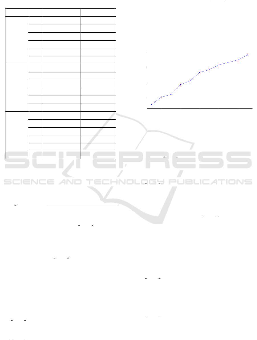
Table 2: The total operating cost difference between the
proposed strategy and the precognition strategy in differ-
ent experiment settings. CompInApp: Compute-intensive
application; BandInApp: Bandwidth-intensive application.
#User T CompInApp BandInApp
3
1 0 0
3 0.05 0.05
5 0.07 0.07
10 0.05 0.08
20 0.05 0.02
30 0.05 0.01
5
1 0 0
3 0.03 0.02
5 0.02 0.03
10 0.05 0.07
20 0.02 1.5e−3
30 0.01 0.01
10
1 0 0
3 0.04 0.03
5 0.05 0.06
10 4.8e−3 4.4e−3
20 0.03 0.03
30 0.03 0.02
tor parameter to 0.995, to ensure it obtains a solution
within a reasonable amount of time. We collect the re-
sults obtained from both algorithms and calculate the
deviation in total operating costs using the following
formula:
cost difference =
cost
(proposed)
− cost
(precognition)
cost
(precognition)
In Table 2, we show the differences in total operat-
ing costs achieved with the App EDC Match strat-
egy and the precognition strategy across different set-
tings of numbers of users (i.e., 3, 5, and 10 users)
and time window lengths (i.e., 1, 3, 5, 10, 20, and
30 time slots). As observed, the total operating costs
achieved with the App EDC Match placement strat-
egy are pretty close to the approximate optimal val-
ues returned by the precognition strategy, with a max-
imum deviation of approximately 8%.
5.2 What Are The Execution Times of
the Proposed Placement Algorithm?
We now evaluate the scalability of the
App
EDC Match placement strategy and its suit-
ability for real MECs, where real-time decision-
making is crucial. As presented in Section 3, the
App EDC Match strategy’s execution time depends
on the number of EDCs n and the number of users
m, i.e., its time complexity is O(n × m). To verify
that the execution time of App EDC Match scales
linearly with the number of users in a fixed MEC
infrastructure, we measure the mean execution time
per time slot for the proposed strategy with varying
number of users. In essence, we use the same emu-
lated MECs as in previous experiments and increase
the number of users per experiment.
25
50
75
100
1000 2000 3000 4000 5000
# Number of Users
Mean Execution Time Per Time Slot (msec)
Figure 3: Mean execution time per time slot for the pro-
posed online placement strategy with the number of users
ranging from 500 to 5500. The red vertical line connects
the maximum and minimum observed execution times.
Figure 3 shows the mean execution time per time
slot of App EDC Match as the number of users is
raised from 500 to 5500 users. As observed, the exe-
cution time per time slot increases linearly with the
number of users. Moreover, the execution time of
App EDC Match starts off considerably lower but ex-
periences a rapid increase. Nonetheless, the execution
times per time slot remain reasonably small, staying
below 100 ms for the experiment with 5500 users,
which is well below the length of the time slots (1
minute). As a result, the App EDC Match algorithm
is well-suited for deployment in real MEC systems to
rapidly determine placement solutions that approach
the near-global optimum.
5.3 Where Are Applications Placed by
the Proposed Algorithm?
We analyse the results produced by the
App EDC Match placement strategy to better
understand its behavior. Figure 4 shows the dis-
tribution of applications throughout the entire
experiment. For the bandwidth-intensive applica-
tions, to minimize network bandwidth utilization
and thereby reduce overall operational costs, the
App EDC Match strategy prioritizes the placement
of applications on the EDC to which the application’s
users directly connected. Consequently, 91% of
bandwidth-intensive applications are placed on the
State-Aware Application Placement in Mobile Edge Clouds
125
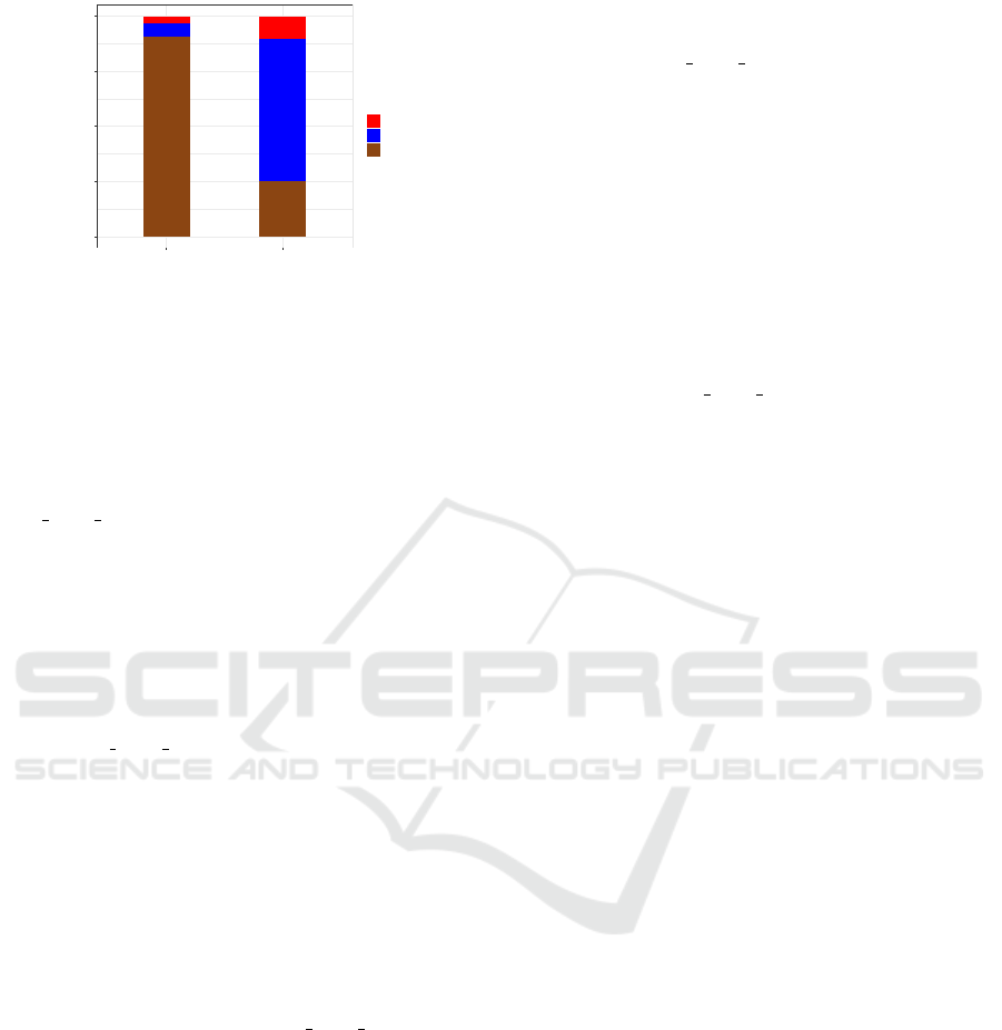
0.00
0.25
0.50
0.75
1.00
BandwidthInt. ComputeInt.
Application Type
Percentage
Place_at
L−3
L−2
L−1
Figure 4: Behavior of the proposed placement strategy
with bandwidth-intensive (BandwidthInt.) and compute-
intensive (ComputeInt.) applications. L-1, L-2, L-3 denote
layers 1, 2, and 3 in the emulated MEC, respectively.
connecting EDCs of the users, while approximately
5.8% are placed on layer 2 EDCs, and the remaining
3.2% being placed on layer 3 EDCs.
In case of compute-intensive applications, the
App EDC Match strategy leverages higher-capacity
resources from EDCs in upper layers, which typi-
cally offer lower compute resources unit prices. More
specifically, approximately 25.1% of the compute-
intensive applications are placed on the EDCs directly
connected to users, while a larger portion, roughly
64.5% are placed on layer 2 EDCs, and the remain-
ing 10.4% of these applications are placed on layer
3 EDCs. These observed results show the effective-
ness of App EDC Match in achieving a balanced and
efficient utilization of resources within MEC infras-
tructure.
Taking the analysis a step further, we investigate
the utilization of compute resources within EDCs
at each layer and the utilization of network band-
width (expressed as a percentage of the total capac-
ity) in network links during a peak workload scenario
characterized by a high volume of concurrent users.
Figure 5 shows the experimental results with com-
pute intensive applications. In the previous exper-
iment, we observed that the App EDC Match strat-
egy effectively distributes compute intensive applica-
tions leveraging the greater computing capabilities of
EDCs in higher layers (layer 2 and 3). As a result, the
workload is not significantly concentrated in EDCs in
layer 1, leading to average resource utilization rates
of 54.2% for EDCs in layer 1, 17.5% for EDCs in
layer 2, and 11.4% for EDCs in layer 3 (Figure 5a).
Regarding bandwidth usage, we observe an average
bandwidth usage of 11.9% on the links connecting
layer 2 and layer 3, while the links connecting layers
1 and 2 exhibited an average bandwidth utilization of
18.3% (Figure 5b).
Figure 6 presents the experimental results related
to bandwidth-intensive applications. Since these ap-
plications demand fewer compute resources, we ob-
serve that the App EDC Match strategy primarily uti-
lizes compute resources from EDCs in layer 1. This
results in an average resource usage of 24.8% for
EDCs in this layer, while the corresponding values
for EDCs in layers 2 and 3 are 1.3% and 0.8%, re-
spectively (Figure 6a). Consequently, this applica-
tion placement pattern impacts bandwidth usage in
the network links. There is a higher concentration of
bandwidth utilization on the links connecting layer 1
and layer 2, with an average of 3.9%. In contrast,
the links between layer 2 and layer 3 demonstrate
less concentrated bandwidth usage, averaging 1.1%
(Figure 6b). These results not only show the effec-
tiveness of the App EDC Match placement strategy,
but also provide further confirmation of the findings
in (Mehta et al., 2016), which underscore the advan-
tages of introducing intermediate layers of EDCs, in-
cluding cost savings, prevention of compute capacity
shortages, and the mitigation of network congestion
within MECs environment.
6 RELATED WORK
In this section, we explore research efforts addressing
the MEC application placement problem.
Ouyang et al. (Ouyang et al., 2019) introduced an
online service placement method for MECs, priori-
tizing user latency and service migration cost. Their
approach utilizes a Thompson-sampling based on-
line learning algorithm to adaptively select service
locations based on user preferences, resulting in im-
proved performance compared to alternative methods,
as demonstrated through theoretical analysis and per-
formance evaluation. Farhadi et al. (Farhadi et al.,
2021) introduced a two-time-scale framework for op-
timizing service placement and request scheduling,
considering various constraints. Their algorithms
demonstrated efficient polynomial-time performance
and consistently achieved high optimization levels.
Similarly, Gao et al. (Gao et al., 2021) addressed on-
line service placement in MECs, dividing it into se-
lecting the access network and determining service
deployment locations. They aimed to enhance QoS by
balancing factors like access and communication de-
lays, using an iterative-based algorithm to approach
optimality. Smolka et al. (Smolka et al., 2023) pro-
posed a decentralized method for dynamic edge ap-
plication placement. Each edge node autonomously
decides through auctions to minimize application la-
tency individually.
These previous works primarily focus on high-
CLOSER 2024 - 14th International Conference on Cloud Computing and Services Science
126
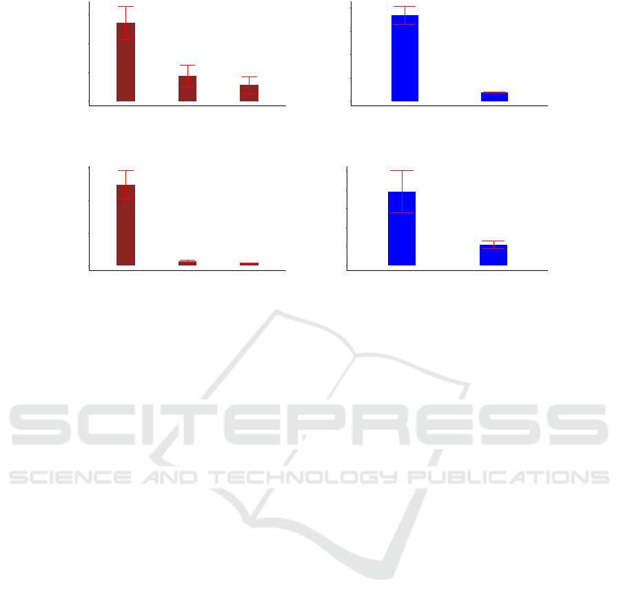
0
20
40
60
L−1 L−2 L−3
Layer
Average Resource Usage %
a Compute resource usage.
0
5
10
15
20
L−1 to L−2 L−2 to L−3
Network Link
Average Bandwidth Usage %
b Bandwidth usage.
Figure 5: Experiment with compute-intensive applications.
0
10
20
30
L−1 L−2 L−3
Layer
Average Resource Usage %
a Compute resource usage.
0
1
2
3
4
5
L−1 to L−2 L−2 to L−3
Network Link
Average Bandwidth Usage %
b Bandwidth usage.
Figure 6: Experiment with bandwidth-intensive applications.
level abstractions of applications and are most effi-
cient when dealing with general, stateless applica-
tions. Our work builds upon these existing efforts,
particularly in understanding the cost components as-
sociated with application placement operations. Nev-
ertheless, we incorporate additional aspects to our
approach to the problem. Firstly, we consider dy-
namic workloads that vary from one time slot to an-
other. Secondly, we explicitly incorporate data ex-
change costs, especially the bandwidth cost, along the
network path connecting the EDC co-located with the
nearest tower to the end-user and the EDC responsible
for managing the end-user’s workload.
7 CONCLUSION AND FUTURE
WORK
In this paper, we tackle the challenge of deploy-
ing stateful applications in MEC environments. Our
approach begins with a comprehensive modeling of
the anticipated workloads, applications, and MEC in-
frastructures. Subsequently, we define and analyze
the various costs associated with application opera-
tion, encompassing resource utilization costs, migra-
tion cost, and the costs incurred due to service qual-
ity degradation. Lastly, we introduce an efficient on-
line placement algorithm driven by the Gale-Shapley
matching algorithm. The experiments reveal that the
proposed algorithm enables MECs to make swift de-
cisions on allocating capacity for applications, result-
ing in total operating costs that are no more than 8%
higher than the approximate global optimum obtained
from an offline precognition algorithm. Moreover, it
effectively facilitates workload balancing, mitigating
resource scarcity challenges for MECs.
We envision several promising directions for fu-
ture research. While the proposed placement algo-
rithm treats all applications equally, it is essential
to acknowledge that real-world scenarios often in-
volve mission-critical applications with strict local-
ity requirements. These applications necessitate be-
ing hosted on resources from EDCs in close proxim-
ity to end-users. As a result, we intend to enhance
the application model presented in this study to incor-
porate application priorities. Subsequently, we will
adapt our proposed placement algorithms to account
for these priority considerations. Secondly, we plan
to explore distributed placement algorithms designed
for deployment across all EDCs. Ideally, these dis-
tributed algorithms should exhibit execution times in-
dependent of the number of EDCs. This investiga-
tion aims to further optimize and scale our placement
strategies in large-scale MEC environments.
ACKNOWLEDGEMENTS
This work was partially supported by the Knut
and Alice Wallenberg Foundation, both directly and
through the Wallenberg AI, Autonomous Systems
and Software Program (WASP), as well as by the
State-Aware Application Placement in Mobile Edge Clouds
127

eSSENCE strategic research programme.
REFERENCES
Apat, H. K., Nayak, R., and Sahoo, B. (2023). A com-
prehensive review on internet of things application
placement in fog computing environment. Internet of
Things, page 100866.
Bartolomeo, G., Yosofie, M., B
¨
aurle, S., Haluszczynski,
O., Mohan, N., and Ott, J. (2023). Oakestra: A
lightweight hierarchical orchestration framework for
edge computing. In 2023 USENIX Annual Technical
Conference (USENIX ATC 23), pages 215–231.
Cardellini, V., Nardelli, M., and Luzi, D. (2016). Elastic
stateful stream processing in storm. In 2016 Interna-
tional Conference on High Performance Computing &
Simulation (HPCS), pages 583–590. IEEE.
Dally, W. J. and Towles, B. P. (2004). Principles and prac-
tices of interconnection networks. Elsevier.
Ellis, S. R., Mania, K., Adelstein, B. D., and Hill, M. I.
(2004). Generalizeability of latency detection in a
variety of virtual environments. In Proceedings of
the Human Factors and Ergonomics Society Annual
Meeting, volume 48, pages 2632–2636. SAGE Publi-
cations Sage CA: Los Angeles, CA.
Farhadi, V., Mehmeti, F., He, T., La Porta, T. F., Kham-
froush, H., Wang, S., Chan, K. S., and Poularakis, K.
(2021). Service placement and request scheduling for
data-intensive applications in edge clouds. IEEE/ACM
Transactions on Networking, 29(2):779–792.
Fisher, M. L., Jaikumar, R., and Van Wassenhove, L. N.
(1986). A multiplier adjustment method for the gen-
eralized assignment problem. Management science,
32(9):1095–1103.
Gale, D. and Shapley, L. S. (1962). College admissions and
the stability of marriage. The American Mathematical
Monthly, 69(1):9–15.
Gao, B., Zhou, Z., Liu, F., Xu, F., and Li, B. (2021). An on-
line framework for joint network selection and service
placement in mobile edge computing. IEEE Transac-
tions on Mobile Computing, 21(11):3836–3851.
Kavak, N., Wilkinson, A., Larkins, J., Patil, S., and Frazier,
B. (2015). The central office of the ict era: Agile,
smart, and autonomous. Ericsson Technol. Rev, 93:1–
13.
Li, R., Zhou, Z., Zhang, X., and Chen, X. (2022). Joint
application placement and request routing optimiza-
tion for dynamic edge computing service manage-
ment. IEEE Transactions on Parallel and Distributed
Systems, 33(12):4581–4596.
Mehta, A., T
¨
arneberg, W., Klein, C., Tordsson, J., Kihl,
M., and Elmroth, E. (2016). How beneficial are inter-
mediate layer data centers in mobile edge networks?
In 2016 IEEE 1st International Workshops on Foun-
dations and Applications of Self* Systems (FAS* W),
pages 222–229. IEEE.
Moore, H. L. (1925). A Moving Equilibrium of Demand
and Supply. The Quarterly Journal of Economics,
39(3):357–371.
Moudi, M. and Othman, M. (2020). On the relation between
network throughput and delay curves. Automatika,
61(3):415–424.
Nguyen, C., Klein, C., and Elmroth, E. (2019). Multivari-
ate lstm-based location-aware workload prediction for
edge data centers. In 2019 19th IEEE/ACM Interna-
tional Symposium on Cluster, Cloud and Grid Com-
puting (CCGRID), pages 341–350. IEEE.
Observer Analytics (2022). Average session time of vr users
in the US q2 - q3 2019, by user type. Accessed on
12/12/2023.
Ouyang, T., Li, R., Chen, X., Zhou, Z., and Tang, X.
(2019). Adaptive user-managed service placement for
mobile edge computing: An online learning approach.
In IEEE INFOCOM 2019-IEEE Conference on Com-
puter Communications, pages 1468–1476. IEEE.
Pantel, L. and Wolf, L. C. (2002). On the impact of delay
on real-time multiplayer games. In Proceedings of the
12th international workshop on Network and operat-
ing systems support for digital audio and video, pages
23–29.
Piorkowski, M., Sarafijanovoc-Djukic, N., and Gross-
glauser, M. (2009). CRAWDAD dataset epfl/mobility
(v. 2009-02-24). Downloaded from https://crawdad.
org/epfl/mobility/20090224.
Shang, X., Huang, Y., Mao, Y., Liu, Z., and Yang, Y. (2022).
Enabling qoe support for interactive applications over
mobile edge with high user mobility. In IEEE INFO-
COM 2022-IEEE Conference on Computer Commu-
nications, pages 1289–1298. IEEE.
Smolka, S., Wißenberg, L., and Mann, Z.
´
A. (2023).
Edgedecap: An auction-based decentralized algo-
rithm for optimizing application placement in edge
computing. Journal of Parallel and Distributed Com-
puting, 175:22–36.
Tong, L., Li, Y., and Gao, W. (2016). A hierarchical edge
cloud architecture for mobile computing. In IEEE IN-
FOCOM 2016-The 35th Annual IEEE International
Conference on Computer Communications, pages 1–
9. IEEE.
Van Laarhoven, P. J. and Aarts, E. H. (1987). Simulated
annealing. In Simulated annealing: Theory and ap-
plications, pages 7–15. Springer.
Wang, S., Zafer, M., and Leung, K. K. (2017). Online place-
ment of multi-component applications in edge com-
puting environments. IEEE Access, 5:2514–2533.
Yang, B., Chai, W. K., Xu, Z., Katsaros, K. V., and Pavlou,
G. (2018). Cost-efficient nfv-enabled mobile edge-
cloud for low latency mobile applications. IEEE
Transactions on Network and Service Management,
15(1):475–488.
CLOSER 2024 - 14th International Conference on Cloud Computing and Services Science
128
