DeepTraderX: Challenging Conventional Trading Strategies with Deep

Learning in Multi-Threaded Market Simulations

Armand Mihai Cismaru

Department of Computer Science, University of Bristol, Woodland Road, Bristol, U.K.

Keywords:

Algorithmic Trading, Deep Learning, Automated Agents, Financial Markets.

Abstract:

In this paper, we introduce DeepTraderX (DTX), a simple Deep Learning-based trader, and present results

that demonstrate its performance in a multi-threaded market simulation. In a total of about 500 simulated

market days, DTX has learned solely by watching the prices that other strategies produce. By doing this, it

has successfully created a mapping from market data to quotes, either bid or ask orders, to place for an asset.

Trained on historical Level-2 market data, i.e., the Limit Order Book (LOB) for speciﬁc tradable assets, DTX

processes the market state S at each timestep T to determine a price P for market orders. The market data

used in both training and testing was generated from unique market schedules based on real historic stock

market data. DTX was tested extensively against the best strategies in the literature, with its results validated

by statistical analysis. Our ﬁndings underscore DTX’s capability to rival, and in many instances, surpass, the

performance of public-domain traders, including those that outclass human traders, emphasising the efﬁciency

of simple models, as this is required to succeed in intricate multi-threaded simulations. This highlights the

potential of leveraging ”black-box” Deep Learning systems to create more efﬁcient ﬁnancial markets.

1 INTRODUCTION

Recent advancements in computing have catalysed

profound transformations in Artiﬁcial Intelligence

(AI), which now permeates many facets of our daily

lives.

One area impacted by this transformation is the

ﬁnancial sector, or more speciﬁcally, ﬁnancial mar-

kets. They are made up of traders, whether hu-

man or machine, with the core objective of being as

proﬁtable as possible. We call ”algorithmic traders”

the software-driven entities that have replaced human

traders, performing based on pre-deﬁned, complex al-

gorithms derived from complex ﬁnancial engineering.

As markets and technology evolve together, the need

for adaptability to ﬂuctuating conditions is of fore-

most importance. Enter the age of AI traders: more

efﬁcient, enabled to make decisions based on instan-

taneous data analysis, and navigating markets better

than their predecessors.

However, the true paradigm shift is heralded by

the rise of Deep Learning. Its changing potential

is evident across sectors, from chatbots to advanced

medical diagnostics. Deep Learning Neural Networks

https://orcid.org/0009-0007-6374-4639

(DLNNs), modelled after human neural pathways

(Shetty et al., 2020), are at the forefront of this AI

revolution. Their applications span diverse domains

such as speech recognition, natural language process-

ing, and even cancer detection (Abed, 2022). Re-

cent studies underscore the effectiveness of DLNN-

based traders, which have demonstrated capabilities

rivalling, if not exceeding, traditional algorithmic

traders (Calvez and Cliff, 2018). Moreover, the rapid

democratisation of computational power has led to in-

creasingly sophisticated market simulations, enabling

a vast number of research prospects — especially for

the AI community.

Algorithmic traders execute the most of daily

trades in a market, processing millions of transactions

at sub-second rates. While much of the existing lit-

erature evaluates trading strategies in simpliﬁed mar-

ket simulations, the intricate and asynchronous nature

of real-world ﬁnancial markets often remains unad-

dressed. The purpose of this work is to bridge this

research gap in the literature with these core contribu-

tions:

• Train an intelligent trader based on a proven

DLNN architecture on historical simulated data.

• Integrate our trader in an asynchronous market

simulator to enable a solid experiment base.

412

Cismaru, A.

DeepTraderX: Challenging Conventional Trading Strategies with Deep Learning in Multi-Threaded Market Simulations.

DOI: 10.5220/0012355100003636

Paper published under CC license (CC BY-NC-ND 4.0)

In Proceedings of the 16th International Conference on Agents and Artiﬁcial Intelligence (ICAART 2024) - Volume 3, pages 412-421

ISBN: 978-989-758-680-4; ISSN: 2184-433X

• Evaluate our trader against other traders in the lit-

erature based on proﬁts obtained.

• Validate the results through statistical analysis and

reﬂect on the model’s strengths and weaknesses.

The core contribution is creating a system that

could outperform existing strategies in a multi-

threaded market simulator. A positive result could

have an impact in the real world, with the only bar-

rier represented by the access to some of the LOB

data the model requires. Customer limit prices are not

public when trading, so owning such historical data

would prove to be great leverage. In the case of a

negative result, this research would prove useful un-

derlying causes and ascertain the vulnerabilities that

a DLNN trader has when deployed in a realistic set-

ting, albeit with the caveat of accessing certain propri-

etary LOB data. Our exploration is both an homage

and an extension of the efforts of two previous pieces

of research, DeepTrader (Wray et al., 2020) and the

Threaded Bristol Stock Exchange (TBSE) (Rollins

and Cliff, 2020), seeking to chart new horizons in the

conﬂuence of AI and ﬁnancial trading.

1.0.1 Context on Financial Markets and

Algorithmic Traders

Over the course of this paper, there are a number of

specialised terms and concepts relevant to our work,

especially regarding the LOB, which are going to be

expanded on in the following sub-section.

At the core of most ﬁnancial markets lies the Con-

tinuous Double Auction (CDA) mechanism (Smith,

1962). Unlike the traditional auction setup, where

items are sold one at a time with bidders actively

competing until the highest price is reached, the CDA

operates continuously, allowing buyers and sellers to

place orders at any time. The ”double” in CDA signi-

ﬁes that it facilitates both buying and selling, dynami-

cally matching buy orders with corresponding sell or-

ders based on price preferences.

Central to the operation of the CDA is the LOB.

The LOB is a dynamic, electronic record of all the

outstanding buy and sell orders in the market for a

particular asset. These orders are organised by price

level, with the ”bid” price representing the maximum

amount a buyer is willing to pay and the ”ask” price

indicating the minimum amount a seller is willing to

accept. The difference between the highest bid and

the lowest ask is known as the ”spread”. A key fea-

ture of the LOB is that orders are processed based on

price-time priority. This means that orders at the best

price are always executed ﬁrst, and among orders at

the same price, the one placed earlier gets priority. In

a typical market scenario, traders—either humans or

algorithms—submit orders. These orders can be of

two main types:

• Limit Orders: A trader is given a price and quan-

tity. For buyers, this price is the maximum they’re

willing to pay, and for sellers, it’s the minimum

they’re willing to accept. These orders are added

to the LOB, waiting for a matching order to arrive.

• Market Orders: A trader speciﬁes only the quan-

tity, aiming to buy or sell immediately at the best

available price. These orders are not added to

the LOB; instead, they are matched with the best

available opposite order from the LOB.

The market’s primary objective is to facilitate

trading by matching buy and sell orders. The continu-

ous updating and matching in the LOB ensure liquid-

ity and dynamic price discovery, reﬂecting the current

consensus value of an asset.

The data we require from the LOB is referred to

as ”Level-2” data, meaning that we get all the current

active orders. For context, ”Level-1” market data con-

tains only the prices and quantities of the best bid and

ask in the market.

The TBSE is an advanced, asynchronous version

of the open-source Bristol Stock Exchange (BSE)

(Cliff, 2022), a faithful, detailed simulation of a ﬁ-

nancial exchange where a variety of public-domain

automated trading algorithms interact via a CDA. It is

asynchronous in the way traders interact with the mar-

ket, with each trying to buy or sell an asset by plac-

ing Limit Orders concomitantly. Abiding by Smith’s

guidelines (Smith, 1962), traders solely aim for proﬁt,

ensuring no trades occur at a loss. Unlike its predeces-

sor, where traders were sequentially polled for orders,

TBSE grants each trader its own thread. Throughout

a market session, traders continuously receive market

updates and decide on placing orders. This structure

privileges faster algorithms, as orders are queued on a

”ﬁrst in, ﬁrst out” (FIFO) basis, emulating real-world

market dynamics more closely.

The following terms will be relevant when deﬁn-

ing our model’s features. The LOB midprice is the

average of the highest bid and the lowest ask prices

in the LOB. The microprice reﬁnes this midprice by

factoring in the order imbalance and the depth of the

order book. Imbalance represents the proportionate

difference between buy and sell orders, highlighting

directional pressure. Total quotes on the LOB refer to

the aggregate of all buy and sell orders present. The

estimate P∗ of the competitive equilibrium price pre-

dicts where supply meets demand, ensuring market

clearance. Lastly, Smith’s ”alpha” α metric gauges

how closely the market price approaches this equilib-

rium, serving as a measure of market efﬁciency.

DeepTraderX: Challenging Conventional Trading Strategies with Deep Learning in Multi-Threaded Market Simulations

413

Now having cleared the domain-speciﬁc con-

text, we transition to showing how experimental eco-

nomics evolved from Smith’s inaugural work to AI al-

gorithmic traders, understanding how our work builds

on existing knowledge in Section 2. The rest of this

paper, based on (Cismaru, 2023), will detail how the

model that DTX uses was trained and the experimen-

tal setup in Section 3. The results showing how DTX

outperforms existing traders are shown in Section 4.

Section 5 will further analyse these ﬁndings, with

Section 6 providing a view on limitations and future

work, concluding with Section 7. (OpenAI, 2023)

2 BACKGROUND

2.0.1 Beginnings of Experimental Economics

and Agent Based Modelling

The groundwork for experimental economics was laid

by Vernon Smith in 1962 by publishing ”An Ex-

perimental Study of Competitive Market Behaviour”

in The Journal of Political Economy (JPE) (Smith,

1962). Smith has implemented a series of experi-

ments based on the CDA system, where buyers and

sellers are announcing bids and others in real-time,

with the possibility of a trade being executed any time

the prices match.

The experiments were performed with small

groups of human traders. They were instructed to

trade an arbitrary commodity on an open-pit trading

ﬂoor with the intention of maximising proﬁtability,

namely the difference between the limit price and the

trade price. Each trader was given a pre-deﬁned limit

price: for sellers, the minimum they are allowed to

sell their units at, and for buyers, the maximum price

they can pay for a unit of the traded asset, thus pre-

venting loss-making trades. The simulations were

carried out as ”trading days”, namely time intervals

of 5 to 10 minutes. The quotes that were shouted by

the traders resembled the LOBs of modern markets.

Once a trader agreed on a trade with its counterparty,

both would leave the market as they only had a sin-

gle unit to trade. The results showed rapid conver-

gence to the theoretical equilibrium price, measured

by Smith’s α metric. It measures how well and ef-

ﬁciently the market is converging to the equilibrium

price. The experiments capture the asynchronous na-

ture of ﬁnancial markets, one of the issues that this

work is aiming to explore. Vernon Smith received the

Nobel Prize in 2002 for his pioneering work in exper-

imental economics, with his experiment styles being

the basis of most research carried out in this ﬁeld and

the methodology used in this paper.

Three decades later, in 1993, Gode and Sunder

introduced the Zero Intelligence traders (Gode and

Sunder, 1993). Their focus is on studying how auto-

mated traders perform in markets dominated by hu-

man traders. They introduced two trading strate-

gies: Zero Intelligence Unconstrained (ZIU) and Zero

Intelligence Constrained (ZIC). ZIU is generating

purely random quotes, while ZIC is limited, con-

strained to a price interval. Their experiments, car-

ried out in the style of Vernon Smith, showed ZIC

to outperform human traders. A few years later, in

1997, Cliff published a paper proposing Zero Intel-

ligence Plus (ZIP) traders, which, by using a simple

form of Machine Learning (ML), can be adaptive and

converge in any market condition (Cliff, 1997). ZIP is

based on a limit price and an adaptive proﬁt margin.

The margin is inﬂuenced by a learning rule and the

conditions of the market.

In 1998, Gjerstad & Dickhaut described an adap-

tive agent, GD (Gjerstad and Dickhaut, 1998), with

Tesauro & Bredin publishing a paper in 2002 de-

scribing the GD eXtended (GDX) trading algorithm

(Tesauro and Bredin, 2002). In 2006, Vytelingum’s

thesis introduced what is called the Aggressive-

Adaptive (AA) strategy (Vytelingum, 2006), which

was thought to be the best-performing agent until re-

cently. In 2019, Cliff and Snashall performed com-

prehensive experiments comparing AA and GDX,

simulating over a million markets. The results show

that AA is routinely outperformed by GDX, argu-

ing that advancements in cloud computing and com-

pute power open new possibilities for strategy evalua-

tion that were not possible before (Snashall and Cliff,

2019).

2.0.2 Rise of Intelligence in Market Modelling

and Price Prediction

The advent of AI has attracted the attention of the ﬁ-

nance and trading ﬁelds. Increasing numbers of pa-

pers detail how advanced Deep Learning methods be-

came powerful tools in the world of agent-based trad-

ing, market making, and price forecasting. In their

report, Axtell and Farmer argue that the advance in

computing has enabled agent-based trading (ABM),

impacting how trading is performed today (Axtell and

Farmer, 2018). In ﬁnance, ABM helped us under-

stand markets, volatility, and risk better. Their report

is comprehensive and can be considered a higher-level

point of reference on how agents are applied in differ-

ent branches of ﬁnance and economics. Njegovanovi

published a paper in 2018 that discusses the implica-

tions of AI in ﬁnance, with a focus on how the human

brain and its behaviour have inspired the architecture

of automatic decision models (Njegovanovi

c, 2018).

ICAART 2024 - 16th International Conference on Agents and Artiﬁcial Intelligence

414

In the past decade, a number of studies have ex-

plored the potential of Deep Learning in ﬁnance. In

2013, Stotter, Cartlidge, and Cliff introduced a new

method for assignment adaptation in ZIP, performing

balanced group tests against the well-known ZIP and

AA strategies (Stotter et al., 2013). Their results show

that assignment-adaptive (ASAD) traders equilibrate

more quickly after market shocks than base strategies.

In 2020, Silva, Li, and Pamplona use LSTM-based

trading agents to predict future trends in stock in-

dex prices. Their proposed method, named LSTM-

RMODV, demonstrates the best performance out of

all studied methods, and it is shown to work in both

bear and bull markets (Silva et al., 2020). In 2019,

Sirignano and Cont proposed a Deep Learning model

applied to historic US equity markets. The informa-

tion extracted from the LOBs uncovers a relationship

between past orders and the direction of future prices.

They conclude that this is better than specialised pre-

dictions for speciﬁc assets. Their results illustrate

the applicability and power of Deep Learning meth-

ods in modelling market behaviour and generalisation

(Sirignano and Cont, 2019).

2.0.3 Need for Intelligence and Realistic

Modelling

The work in this paper continues what Calvez and

Cliff started in 2018 (Calvez and Cliff, 2018), when

they introduced a DLNN system trained to replicate

adaptive traders in a simulated market. Purely based

on the observation of the best bid and ask prices, the

DLNN has managed to perform better than the trader

observed. In 2020, Wray, Meades, and Cliff will take

this further by introducing the ﬁrst version of Deep-

Trader, a high-performing algorithmic trader (Wray

et al., 2020) trained to perform in a sequential mar-

ket. Based on a LSTM, it automatically replicates a

successful trader by training on 14 features derived

from Level-2 market data. The ﬁrst version of Deep-

Trader matches or outperforms existing trading algo-

rithms in the public-domain literature. Most studies

are performed on sequential simulations, in which the

speed at which the traders react to changes in the mar-

ket does not matter. Axtell and Farmer argue in their

above-mentioned report, that the real social and eco-

nomic worlds are parallel and asynchronous, but we

try to replicate it with single-threaded code (Axtell

and Farmer, 2018). Rollins and Cliff try to mitigate

this in a paper they published in 2020 (Rollins and

Cliff, 2020). They propose TBSE, as we introduced in

Section 1.0.1, on which they perform pair-wise exper-

iments between well-known trading strategies. The

results reported intriguing insights, with a new domi-

nance hierarchy of trading algorithms emerging.

Our work aims to integrate an optimised version

of DeepTrader in TBSE and test it againts existing

strategies. We will dive into the details of this in the

next section, asking the question: Can we train this

model to learn from a variety of traders and conditions

and study its behaviour in a parallel simulation? We

hope that the results of our study can provide more

insight into its potential real-world performance.

3 METHODS

The core of our work relies on TBSE, as introduced

in Section 1.0.1. It was used to generate the large

amounts of data required for training DTX when run-

ning against the other public-domain trading strate-

gies. The code of our project is available online at

GitHub at github.com/armandcismaru/DeepTraderX

for easy reproducibility.

The market is deﬁned by the the limit orders given

to traders, based on supply and demand schedules.

TBSE was designed to use stochastically-altered real-

world historical data to create variable, more realistic

schedules. For our training and experiment sessions,

we used IBM stock data from the August 31, 2017

NYSE trading day, namely the best/worst bids/asks at

1 minute intervals.

TBSE provides the means to produce large quan-

tities of ”historical” market data. The one metric we

are looking to evaluate DTX on is the mean proﬁt

that each trader type achieves at the end of the ses-

sion, namely proﬁt per trader (PPT). We cannot assess

these algorithmic traders the same way we would with

real traders, as TBSE doesn’t simulate loss, so we are

judging based on proﬁts only.

The data to train the DLNN model is curated by

taking ”snapshots” of the Level-2 LOB data, updated

each time a trade occurs. During training, our DLNN-

based trader is given 14 numeric inputs, deriving from

these LOB snapshots, as detailed in Section 1.0.1.

The 14 values are as follows:

1. The time t of the trade when it took place.

2. The type of customer order used to initiate the

trade, either a ”bid” or an ”ask” order.

3. The limit price of the trader’s quote that initiated

the trade.

4. The midprice of the LOB at time t.

5. The microprice of the LOB at time t.

6. The LOB imbalance at time t.

7. The spread of the LOB at time t.

8. The best (highest) bid on the LOB at time t.

DeepTraderX: Challenging Conventional Trading Strategies with Deep Learning in Multi-Threaded Market Simulations

415

9. The best (lowest) ask on the LOB at time t.

10. The difference between the current time and the

time of the previous trade.

11. The quantity of all quotes on the LOB at time t.

12. An estimate P

∗

of the competitive equilibrium

price.

13. Smith’s α metric using the P

∗

estimate of the com-

petitive equilibrium price at time t.

14. The target variable: the price of the trade.

When performing inference, our model takes in

the ﬁrst 13 multivariate inputs to produce the target

variable, item 14, namely the price at which it is will-

ing to trade at a speciﬁc time in the market (the quote

placed by the trader).

3.0.1 Data Generation and Preprocessing

TBSE provided ﬁve working trading agents that

were used to generate the training data, as

included here: github.com/MichaelRol/Threaded-

Bristol-Stock-Exchange. To create a large and diver-

siﬁed training dataset, the market simulations were

run using 5 types of traders in different proportions,

with a total of 40 traders per simulation. The follow-

ing proportion-groups of 20 traders per side of the ex-

change (buyers or sellers) were used: (5, 5, 5, 5, 0),

(8, 4, 4, 4, 0), (8, 8, 2, 2, 0), (10, 4, 4, 2, 0), (12, 4,

2, 2, 0), (14, 2, 2, 2, 0), (16, 2, 2, 0, 0), (16, 4, 0, 0,

0), (18, 2, 0, 0, 0), and (20, 0, 0, 0, 0). Each number

in a speciﬁc position corresponds to a population of

traders of a certain type for a market simulation. For

example, for the speciﬁcation (12, 4, 2, 2, 0), there

are 12 ZIC, 4 ZIP, 2 GDX, 2 AA, and no Giveaway

traders for both the buyers and sellers sides.

Using all the unique permutations of the propor-

tions resulted in 270 trader schedules, in which the

5 traders participate equally. This ensured that the

model trains to generalise from a varied and rich set

of market scenarios. Each schedule was executed for

44 individual trials, amounting to 270 × 44 = 11880

market sessions. Each simulation represents one mar-

ket hour, requiring roughly one minute of wall-clock

time. If running on a single computer, generating this

amount of data would require approximately 8.6 days

of continuous execution, generating roughly 13 mil-

lion LOB snapshots. To address this time constraint,

the decision was made to use cloud computing to dis-

tribute computation across several worker nodes.

It is generally good practice to normalise the in-

puts of a network due to performance concerns, par-

ticularly for Deep Learning architectures like LSTMs.

Normalising the inputs helps ensure that all features

are contained within a similar range and prevents one

feature from dominating the others. For example,

we have features with different scales, such as the

time, which runs from 0 to 3600, while the quote

type is binary. So by normalising, we only have val-

ues in the [0,1] interval. Doing this ensures improved

convergence of the optimisation algorithm and helps

the model generalise better to new data. The choice

was to use min-max normalisation, given that we are

working with multivariate features derived from ﬁ-

nancial data.

3.0.2 Model Architecture and Training

Contrary to the usual practices for training and vali-

dating a DLNN, which consist of splitting the dataset

into training, validation, and test subsets, we used all

the dataset for training. Markets are a combination

of unique factors, so our trader’s proﬁt is heavily de-

pendent on what is happening in a speciﬁc simula-

tion. Considering this, it is without purpose to as-

sess its performance relative to historic data by judg-

ing the absolute values of our target variable. Rather,

as the model produced a good drop in the loss level

during training, the DLNN was validated by quantify-

ing how well DTX performed in live market simula-

tions against other traders in terms of PPT. Our dataset

is large and was generated using unique simulations;

thus, DTX doesn’t learn to replicate speciﬁc scenar-

ios; rather, it grows its ability to adapt and generalise

in any condition.

The architecture of the Deep Learning model that

DTX relies on is illustrated in Figure 1. It is com-

prised of three hidden layers, a LSTM with 10 units

(neurons), and two consequent Dense layers with 5

and 3 units, respectively, all using the Rectiﬁed Linear

Unit (ReLU) activation function. The output layers

use a ”linear” activation function, chosen as suitable

for a continuous output variable.

When dealing with large datasets, training should

be done in batches to accommodate memory limita-

tions and speed up training. Our network accommo-

dates this with a custom data generator based on the

Sequence class, used by Keras to train a model in

batches. To balance accuracy and training times, a

batch size of 16384 was chosen. To to balance poten-

tial overﬁtting and long convergence times we chose

a learning rate of µ = 1.5 × 10

−5

. The DLNN uses

the Adam optimizer for its ability to efﬁciently con-

verge to a good solution, prevention of overﬁtting,

and incorporation of momentum, speeding up learn-

ing and improving generalisation performance. The

model was trained in approximately 22 hours, lever-

aging the GPU clusters of the Blue Crystal 4 super-

computer.

The model was trained for 20 epochs. An epoch

ICAART 2024 - 16th International Conference on Agents and Artiﬁcial Intelligence

416

Figure 1: Architecture diagram for the DLNN model used by DTX.

refers to a single pass of the entire dataset through the

neural network. So, at the end of the training session,

DTX is exposed to 11880 × 20 = 237600 market ses-

sions. With each experiment producing ∼ 1100 LOB

snapshots, DTX is trained using a total of roughly 261

million snapshots. The training error (loss) was calcu-

lated using the Mean Square Error (MSE). The error

decreased considerably during the ﬁrst 4 epochs and

approached 0 in the last epoch with a loss curve re-

sembling an asymptote to the X axis.

3.0.3 Experiment Design and Evaluation

Our aim is to quantify how DTX performs relative to

the other strategies. Finding the right methodology

for doing this is as important as the strategy itself, as

it is essential to isolate market conditions in repeat-

able experiments. Traders are dependent on the be-

havior of other strategies, mandating a controlled lab-

oratory environment that allows quantitative analysis

of their performance. Thus, there are two strategies

used in each experiment: DTX and the others, one by

one. Drawing inspiration from the work of Tesauro

and Das (Tesauro and Das, 2001), we have chosen

two experiment types.

For each, DTX has run in n = 500 independent

market simulations, populated by 40 traders, 20 for

each side, buyer or seller. It is worth specifying that

each set of 50 trials was run on a different cloud

machine, resulting in a broad distribution of proﬁts,

with each using the same seed for functions involv-

ing randomness. This is due to the well-known and

researched issue in computer science, that machines

cannot emulate perfect randomness (Bridle, 2022).

TBSE allows full control of the experiment condi-

tions. The time frame of the simulation, the supply

and demand schedules, and the order interval can all

be controlled to isolate the differences between the

chosen strategies. As we use an asynchronous simu-

lation, we are looking to evaluate DTX based on its

DLNN model’s efﬁciency and capacity to generalise

on LOB data, translating into proﬁts.

The ﬁrst experiment design is the Balanced Group

Tests (BGTs), in which the 20 buyers or sellers are

again evenly split between the two trader types, re-

sulting in 10 DTX traders and 10 traders of another

type for each group. The choice is beneﬁcial as it is

a stochastic-controlled trial method that helps reduce

bias sources and improve the internal validity of the

study. We want to make sure that the traders produce

different proﬁts solely because of their inherent strat-

egy, not noise.

The second type of experiment is the One to Many

tests (OTMs), where the trading strategy that you

want to observe becomes the ”invader” out of a ho-

mogenous population made up of different strategies.

For clarity, this means that 2 instances of DTX will

run alongside 38 traders of a given type. This is par-

ticularly useful as we are trying to see how DTX per-

forms in a market shaped almost entirely by another

trader, capturing its dynamics and producing proﬁts.

For fairness, there is one defecting strategy on both

buyer and seller sides.

The research on the proﬁtability of DTX has been

conducted against four ”competitor” traders: ZIC,

ZIP, GDX, and AA, adding up to eight sets of head-

to-head experiments. These strategies were chosen

as they are the most relevant in the literature, with

AA and ZIP being ”super-human” traders, amongst

the ﬁrst to be proven to outperform humans.

4 RESULTS

The following section presents the results of our ex-

periments, summing 4,000 individual market simula-

tions. The outcome largely supports our research hy-

pothesis, with DTX dominating in 6 out of 8 experi-

ments, with very signiﬁcant differences in PPT for a

number of them.

The results are presented in the form of proﬁt dis-

tribution box plots and scatter plots of individual trial

proﬁts. An extended summary of the results and de-

scription of the statistical signiﬁcance tests conducted

on them can be found in Chapter 3.8 and 4 of (Cis-

maru, 2023). In the box plots, the vertical axis is rep-

resented by PPT across trials. The box represents the

interquartile range, the range between the ﬁrst quartile

and the third quartile. The line inside the box repre-

sents the median of the dataset. The whiskers repre-

sent the data within 1.5 times the interquartile range,

with the diamond-shaped points outside them being

considered outliers from a data distribution point of

DeepTraderX: Challenging Conventional Trading Strategies with Deep Learning in Multi-Threaded Market Simulations

417

view. The scatter plots show individual trials in terms

of PPT obtained by both traders. The line in the scat-

ter plot is a diagonal reference line, where the points

would lie if the proﬁts per trader for both strategies

were equal. Points above the line indicate higher prof-

its achieved by DTX, analogous for the other trader.

The ﬁgures are grouped on experiment and trader

type basis. Each set of two box-plots corresponds

to BGTs and OTMs between DTX and one of the 4

other traders for all experiments. Due to space con-

strains, the scatter plots were chosen for the more in-

teresting experiment results, on a case by case basis.

We present them in the following order: ZIC, ZIP,

GDX, and AA. For each experiment, we performed a

Wilcoxon-signed rank-test with a signiﬁcance level of

95%. The null hypothesis is that there is no statistical

difference between the means of the proﬁts achieved

by the traders. A p-value lower than 0.05 indicates

that we can reject the hypothesis, concluding that one

strategy outperforms the other in a given experiment.

4.0.1 ZIC vs. DTX

Figure 2a shows a narrow difference in means be-

tween ZIC and DTX in the BGTs. The statistical

test for 95% signiﬁcance level has indicated that DTX

is the better strategy of this experiment. In the case

of OTMs, the difference in proﬁts is sensibly larger

for DTX, as seen in the proﬁt distribution in Figure

2b and in the cluster of proﬁts above the diagonal in

Figure 3. The statistical test has conﬁrmed the domi-

nance of DTX in this experiment.

(a) BGTs for ZIC vs. DTX.

(b) OTMs for ZIC vs. DTX.

Figure 2: Box-plots showing PPT for ZIC vs. DTX tests.

4.0.2 ZIP vs. DTX

The BGT experiment between ZIP and DTX is its

only categorical loss. While Figure 5 doesn’t indi-

cate any immediate winner, Figure 4a shows a slight

advantage for ZIP, with a higher mean PPT. The

Wilcoxon signed-rank test has conﬁrmed the result,

conﬁrming that there is a signiﬁcant difference in

Figure 3: Scatter plot of PPT in OTMs for ZIC vs. DTX.

proﬁts in favour of ZIP.

On the other hand, Figure 4b shows higher mean

proﬁts for DTX, although with a much bigger vari-

ance and a number of outlier values, fact backed by

the result of the statistical test.

(a) BGTs for ZIP vs. DTX.

(b) OTMs for ZIP vs. DTX.

Figure 4: Box-plots showing PPT for ZIP vs. DTX tests.

Figure 5: Scatter plot of PPT in BGTs for ZIP vs. DTX.

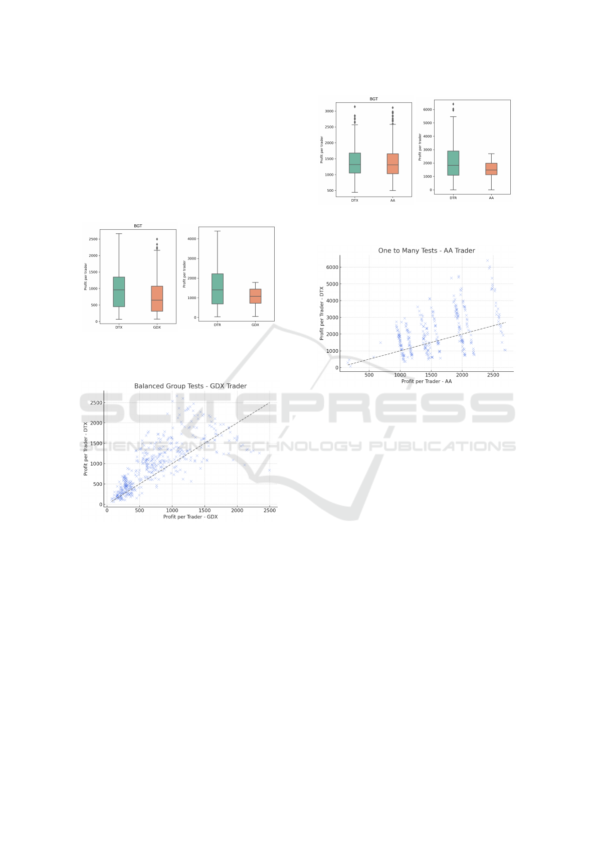
4.0.3 GDX vs. DTX

Figures 6a and 7 show BGT comparison of PPT

scores between DTX and GDX. Upon visual inspec-

tion, the bar plot shows a signiﬁcant difference be-

tween the means of DTX and its competitor, with the

ICAART 2024 - 16th International Conference on Agents and Artiﬁcial Intelligence

418

scatter plot placing most of its points above the diag-

onal, indicating the clear dominance of DTX in this

experiment, with the same outcome conﬁrmed by the

outcome of our statistical test.

Figure 6b shows PPT score comparisons in the

OTM experiment. The proﬁts obtained by DTX, al-

though they have a high variance, lay on a superior

magnitude scale than those of GDX, as visible in the

box-plot. The Wilcoxon signed-rank test conﬁrms

this hypothesis.

(a) BGTs for GDX vs DTX.

(b) OTMs for GDX vs. DTX.

Figure 6: Box-plots showing PPT for GDX vs. DTX tests.

Figure 7: Scatter plot of PPT in BGTs for GDX vs. DTX.

4.0.4 AA vs. DTX

Figure 8a visually represents the proﬁts obtained by

AA and DTX in the BGTs, indicating similar results

for both traders. The statistical test applied failed to

prove that there is a signiﬁcant difference in terms of

mean proﬁts between AA and DTX. Thus, this is our

only inconclusive experiment.

On the other side, Figure 8b shows a high-proﬁt

but high-variance DTX in the OTM experiments

against AA, a fact also visible by looking at the points

above the diagonal in the scatter plot in Figure 9.

The statistical test concludes that DTX is the higher-

performing strategy in this experiment, but with in-

creased variance.

(a) BGTs for AA vs. DTX.

(b) OTMs for AA vs. DTX.

Figure 8: Box-plots showing PPT for AA vs. DTX tests.

Figure 9: Scatter plot of PPT in OTMs for AA vs. DTX.

4.0.5 Summary of Results

The results presented in this section are used to ob-

jectively highlight what a trader based on a simple

LSTM architecture is able to achieve. To recap, our

model was exposed to prices quoted by traders at time

a T and the corresponding LOB state S (as described

in Section 3) during training. The scope of this is to

enable the model to ”read” the market, and, alongside

its own limit price, perform inference and generate a

price used to place a market order. Whether that price

produces proﬁt is down to how quickly (due to the

asynchronous simulation) and accurate DTX reacts to

the market and the behaviour of other traders.

In summary, our empirical analyses reveal that

DTX exhibits superior performance in six out of eight

experiments and matches proﬁts in one out of the

eight. DTX achieves its sole purpose, which is to

make proﬁt. Notably, DTX either matches or sur-

passes the performance of three out of the four traders

tested, including those deemed super-human. Specif-

ically, DTX recorded two victories over GDX and

exhibited a win-tie performance against AA. How-

ever, the results against Cliff’s ZIP are more nuanced;

DTX registered both a victory and a defeat in markets

where both traded concurrently.

As we draw a line at the end of this section, having

DeepTraderX: Challenging Conventional Trading Strategies with Deep Learning in Multi-Threaded Market Simulations

419

presented a detailed analysis of the results, it is worth

noting that DTX produced very interesting results, but

it is still an early development initiative. Although the

performance of DTX is notable, we need to have an

objective stance as we transition into the discussion,

where we will delve deeper into an analysis of these

results. The next section will discuss the strengths

and weaknesses of DTX, relating its performance to

previous results in TBSE, and exploring their broader

impact on the ﬁeld at the intersection of ﬁnance and

artiﬁcial intelligence.

5 DISCUSSION

The biggest strength of our results is the consistent

proﬁtability of DTX across all the experimental se-

tups. This accomplishment is particularly relevant

when considering the volatility of markets, which is

better captured in the multi-threaded simulation that

we use. DTX’s ability to outperform or match traders

such as AA, GDX, or ZIC suggests that the model can

be relied on to trade real money in real markets, gen-

eralising effectively across various scenarios and ag-

gregate on-the-spot information better than humans.

Our trader is not adaptive, so it reacts consistently and

quickly no matter the conditions.

We treat DTX as a ”black-box” trader, so we can-

not explain its inner processes on why it produces a

certain quote price when given its 13 input features,

but we are analysing how those prices produce proﬁts

relative to other traders. The individual prices pro-

duced are almost impossible to interpret by humans,

rather we judge the proﬁts they produce, which are

also a function of how and when the other traders act.

DTX performed the best against ZIC and GDX. While

the results againts ZIC were expected, as it is a sim-

ple, non-adaptive trader, the performance relative to

GDX was impressive in both experiment types. This

result might render the adaptive Dynamic Program-

ming framework that GDX relies on as obsolete when

facing modern DLNN based traders.

However, DTX has matched but not completely

outperformed the ”super-human” traders, AA and

ZIP. In the BGTs againts these two, DTX was less

effective, with a tie and a narrow loss. The simple

ML rule of ZIP and the aggressive pricing system of

AA are still efﬁcient strategies, meaning that DTX is

still ”young”, and not stable enough to dominate in

larger groups. In the OTMs, DTX dominated, being

able to intercept proﬁts as an ”intruder” when running

againts the best traders. The high variance in these ex-

periments suggests that DTX should not be used when

seeking fast proﬁts, but should rather be run in longer

time frames to prove its efﬁciency.

Within the broader academic discourse on trading

algorithms, our ﬁndings resonate with (Wray et al.,

2020). They proposed this DLNN architecture, man-

aging to outperform other strategies, but only trained

it to copy speciﬁc traders in a sequential simula-

tion. When they introduced TBSE (Rollins and Cliff,

2020), Rollins and Cliff proposed the idea that the

traders in the literature might behave differently when

tested in a concurrent simulation that better reﬂects

real markets. Their results challenged the ”status quo”

of the trader dominance hierarchy, ﬁnding that they

now come as follows: ZIP > AA > GDX > ZIC.

By quantifying the difference in results between DTX

and the four traders, we can say that the relative per-

formance of DTX follows the same ranking.

These results have broader implications as they

have proven how, among so many other applications,

AI autonomous agents can generate real money. DTX

is an early proof-of-concept but its ability to be con-

sistent, resilient, and generalise suggests that such

traders could be pivotal in creating fairer and more

efﬁcient markets. However, it’s crucial to consider

that markets populated solely by these intelligent au-

tomated systems might result in inexplicable events

and our inability, as humans, to understand the new

mechanisms of the ﬁnancial markets we rely on.

6 LIMITATIONS & FUTURE

WORK

This study, while comprehensive, is not without lim-

itations. DTX was trained using rich data, but from

only so many traders and scenarios. Also, our ex-

perimental setup was focused on only two types of

traders at a time. Not to mention the considerable

resource overhead involved in data collection, model

training, and testing. Addressing these in future re-

search would offer even more nuanced insights into

DTX’s capabilities. Moreover, an intriguing avenue

for future exploration would be quantifying the corre-

lation between the model’s inference time and perfor-

mance, as well as the degree of impact of each one of

its 14 features.

In practical applications, a ﬁnancial institution en-

gaged in active trading could potentially deploy the

DTX algorithm, provided they have access to exten-

sive historical LOB data as well as their proprietary

trading data. Given that access to limit order prices

(one of the features of DTX, as described in Section

3) is typically restricted to an entity’s own trading op-

erations, DTX could be trained on this comprehensive

dataset, thereby amalgamating the strengths of multi-

ICAART 2024 - 16th International Conference on Agents and Artiﬁcial Intelligence

420

ple established strategies and leveraging vast comput-

ing resources. A market populated with traders like

DTX can be more efﬁcient in allocating resources,

creating a fair and predictable space. (OpenAI, 2023)

7 CONCLUSION

In the rapidly evolving domain of automated trading,

our study emphasises the potential of Deep Learning

trading algorithms. As markets continue to evolve,

the quest for strategies that can adapt and thrive re-

mains paramount, and DTX, as evidenced by our re-

search, stands as a promising proof-of-concept in this

landscape. In the quest for novelty and realism, we

researched this in a distributed market simulation that

has previously overturned the trader dominance hier-

archy, with DTX being consistent with these ﬁndings.

As we stand on the cusp of this new frontier,

it beckons researchers, practitioners, and policymak-

ers alike to collaboratively shape a future where AI-

augmented trading systems contribute to more efﬁ-

cient, stable, and equitable ﬁnancial markets.

ACKNOWLEDGEMENTS

I want to acknowledge the support of my thesis su-

pervisor, Prof. Dave Cliff. Also, ChatGPT (OpenAI,

2023) has helped with putting ideas into words, with

a few parts of this paper written with its aid.

REFERENCES

Abed, A. H. (2022). Deep Learning Techniques For Im-

proving Breast Cancer Detection And Diagnosis. In-

ternational Journal of Advanced Networking and Ap-

plications, 13(06):5197–5214.

Axtell, R. L. and Farmer, J. D. (2018). Agent-Based Mod-

eling in Economics and Finance: Past, Present, and

Future. Journal of Economic Literature.

Bridle, J. (2022). The Crucial Thing a Computer Can’t Do.

http://bit.ly/3QdAxlM.

Calvez, A. l. and Cliff, D. (2018). Deep Learning can Repli-

cate Adaptive Traders in a Limit-Order-Book Finan-

cial Market. 2018 IEEE Symposium Series on Com-

putational Intelligence (SSCI).

Cismaru, A. (2023). Can Intelligence and Speed Make

Proﬁt? A Deep Learning Trader Challenging Exist-

ing Strategies in a Multi-Threaded Financial Market

Simulation. Master’s thesis, University of Bristol.

Cliff, D. (1997). Minimal-Intelligence Agents for Bar-

gaining Behaviors in Market-Based Environments.

Hewlett-Packard Labs Technical Reports.

Cliff, D. (2022). Github - BSE is a Simple Minimal Sim-

ulation of a Limit Order Book Financial Exchange.

https://github.com/davecliff/BristolStockExchange.

Gjerstad, S. and Dickhaut, J. (1998). Price Formation in

Double Auctions. Games and Economic Behavior,

22(1):1–29.

Gode, D. K. and Sunder, S. (1993). Allocative Efﬁciency

of Markets with Zero-Intelligence Traders: Market as

a Partial Substitute for Individual Rationality. Journal

of Political Economy, 101(1):119–137.

Njegovanovi

c, A. (2018). Artiﬁcial Intelligence: Financial

Trading and Neurology of Decision. Financial Mar-

kets, Institutions and Risks.

OpenAI (2023). ChatGPT. https://chat.openai.com.

Rollins, M. and Cliff, D. (2020). Which Trading Agent is

Best? Using a Threaded Parallel Simulation of a Fi-

nancial Market Changes the Pecking-Order.

Shetty, D., C.A, H., Varma, M. J., Navi, S., and Ahmed,

M. R. (2020). Diving Deep into Deep Learning: His-

tory, Evolution, Types and Applications. International

Journal of Innovative Technology and Exploring En-

gineering, 9(3):2835–2846.

Silva, T. R., Li, A. W., and Pamplona, E. O. (2020). Auto-

mated Trading System for Stock Index Using LSTM

Neural Networks and Risk Management. In 2020

IJCNN, pages 1–8. IEEE.

Sirignano, J. and Cont, R. (2019). Universal Features

of Price Formation in Financial Markets: Perspec-

tives from Deep Learning. Quantitative Finance,

19(9):1449–1459.

Smith, V. L. (1962). An Experimental Study of Competi-

tive Market Behavior. Journal of Political Economy,

70(2):111–137.

Snashall, D. and Cliff, D. (2019). Adaptive-Aggressive

Traders Don’t Dominate. Lecture Notes in Computer

Science, pages 246–269.

Stotter, S., Cartlidge, J., and Cliff, D. (2013). Exploring

Assignment-Adaptive (ASAD) Trading Agents in Fi-

nancial Market Experiments. In ICAART (1), pages

77–88.

Tesauro, G. and Bredin, J. L. (2002). Strategic Sequential

Bidding in Auctions Using Dynamic Programming. In

Proceedings of the ﬁrst international joint conference

on Autonomous agents and multiagent systems: part

2, pages 591–598.

Tesauro, G. and Das, R. (2001). High-Performance Bid-

ding Agents for the Continuous Double Auction. In

Proceedings of the 3rd ACM Conference on Electronic

Commerce, pages 206–209.

Vytelingum, P. (2006). The Structure and Behaviour of the

Continuous Double Auction. PhD thesis, University

of Southampton.

Wray, A., Meades, M., and Cliff, D. (2020). Automated

Creation of a High-Performing Algorithmic Trader via

Deep Learning on Level-2 Limit Order Book Data.

2020 IEEE Symposium Series on Computational In-

telligence (SSCI).

DeepTraderX: Challenging Conventional Trading Strategies with Deep Learning in Multi-Threaded Market Simulations

421