Strategies for Classifier Selection Based on Genetic Programming for
Multimedia Data Recognition
Rafael Junqueira Martarelli
1 a
, Douglas Rodrigues
1 b
, Clayton Reginaldo Pereira
1 c
,
Jurandy Almeida
2 d
and Jo
˜
ao Paulo Papa
1 e
1
Department of Computing, S
˜
ao Paulo State University, Bauru, SP, Brazil
2
Department of Computing, Federal University of S
˜
ao Carlos, Sorocaba, SP, Brazil
Keywords:
Ensemble Pruning, Genetic Programming, Fast-CoViAR, Action Classification.
Abstract:
We live in a digital world with an explosion of data in various forms, such as videos, images, signals, and texts,
making manual analysis unfeasible. Machine learning techniques can use this huge amount of data to train
models as an excellent solution for automating decision-making processes such as fraud detection, product
recommendation, and assistance with medical diagnosis, among others. However, training these classifiers
is challenging, resulting in discarding low-quality models. Classifier committees and ensemble pruning have
been introduced to optimize classification, but traditional functions used to fuse predictions are limited. This
paper proposes the use of Genetic Programming (GP) to combine committee members’ forecasts in a new
fashion, opening new perspectives in data classification. We evaluate the proposed method employing several
mathematical functions and fuzzy logic operations in HMDB51 and UCF101 datasets. The results reveal that
GP can significantly enhance the performance of classifier committees, outperforming traditional methods in
various scenarios. The proposed approach improves accuracy on training and test sets, offering adaptability to
different data features and user requirements.
1 INTRODUCTION
In an increasingly digital era, the proliferation of data
in structures such as text, images, audio, and video
is staggering. This data explosion in domains rang-
ing from large organizations like NASA to individ-
ual internet users presents opportunities and chal-
lenges (Statista, 2023). While manual data analysis
was feasible in the early days of computing, the cur-
rent volume of data has rendered this approach im-
practical. This shift has catalyzed the development of
machine learning, a field now integral to extracting
meaningful insights from vast datasets (Zhou, 2021).
A cornerstone of machine learning is the concept
of classifiers, algorithms designed to categorize ob-
jects into distinct classes. Over time, various classi-
fiers have been developed, each suited to specific data
types and problems. However, training these mod-
a
https://orcid.org/0000-0002-5817-050X
b
https://orcid.org/0000-0003-0594-3764
c
https://orcid.org/0000-0002-0427-4880
d
https://orcid.org/0000-0002-4998-6996
e
https://orcid.org/0000-0002-6494-7514
els is often costly in terms of resources, and many of
them are discarded because they fail to meet the re-
quired classification quality (Zhou, 2021).
Ensemble pruning is a promising approach to en-
hance classification effectiveness in light of tradi-
tional classifiers’ limitations. This approach involves
selecting a subset of classifiers to form a commit-
tee, collectively making decisions on classifying ob-
jects. An example of recent advancement in this
field is the Fast-CoViAR (Santos and Almeida, 2020).
This method demonstrates an innovative video classi-
fication technique using an improved version of the
CoViAR (Wu et al., 2018) method, where a set of
12 classifiers across various model types was tested
against the HMDB-51 database. Our work builds
upon this foundation, using those 12 classifiers to il-
lustrate the impact of our novel approach to optimiz-
ing classifier committees.
Traditional methods for collective decision-
making in ensemble pruning often rely on simple av-
erage or weighted average functions (Zhou, 2021).
While these methods are effective in specific scenar-
ios, they fall short of fully exploiting the advanced
capabilities of computational techniques. The field of
788
Martarelli, R., Rodrigues, D., Pereira, C., Almeida, J. and Papa, J.
Strategies for Classifier Selection Based on Genetic Programming for Multimedia Data Recognition.
DOI: 10.5220/0012467600003660
Paper published under CC license (CC BY-NC-ND 4.0)
In Proceedings of the 19th International Joint Conference on Computer Vision, Imaging and Computer Graphics Theory and Applications (VISIGRAPP 2024) - Volume 2: VISAPP, pages
788-795
ISBN: 978-989-758-679-8; ISSN: 2184-4321
Proceedings Copyright © 2024 by SCITEPRESS – Science and Technology Publications, Lda.

computing has far greater potential to discover more
sophisticated and effective functions than just simple
averages or weighted averages. Recognizing this po-
tential, we can leverage the power of Genetic Pro-
gramming (GP) to thoroughly explore the vast space
of possible functions. GP is an efficient tool to navi-
gate through and identify valid functions for the com-
bination and selection of classifiers, offering a more
dynamic and potentially more effective approach than
traditional methods.
This paper proposes a novel application of GP to
optimize the selection of classifiers and the combina-
tion function in ensemble pruning, harnessing the full
potential of computational capabilities in this domain.
Therefore, the main contributions of this work are:
• Using GP to select and combine classifiers in en-
semble pruning innovatively.
• Introducing the concept of optimization of the
combination function in ensemble pruning to the
state of the art.
• Demonstrating the adaptability and efficiency of
GP in handling diverse datasets, showcasing its
ability to improve classification accuracy across
various data types.
• Exploring and contemplating potential functions
for classifier combination contributes to a deeper
understanding of how different functions can en-
hance or affect the performance of ensemble
methods.
The remainder of this paper is organized as fol-
lows: Section 2 delves into the background of Fast-
CoViAR, Ensemble Pruning, and GP. Section 3 de-
scribes the proposed methodology utilizing GP for
ensemble pruning. Section 4 presents our experimen-
tal results, showcasing the effectiveness of the pro-
posed methodology. In Section 5, we conduct an ab-
lation study to further understand the impact of our
approach. The discussion of these results and their
implications is covered in Section 6. Finally, Sec-
tion 7 concludes the paper, summarizing our findings
and suggesting avenues for future research.
2 THEORETICAL BACKGROUND
This section presents a detailed background on the
key concepts relevant to our study, laying the foun-
dation for developing our new classifier selection and
combination method.
2.1 Fast-CoViAR
Santos and Almeida (2020) introduced an innovative
approach to video classification using an improved
version of the CoViAR method, named Fast-CoViAR.
Its significant contribution concerns training a set of
12 classifiers across four model types and their testing
on distinct divisions of the HMDB-51 database (San-
tos and Almeida, 2020). These classifiers provide
a practical framework for our study, as we aim to
demonstrate the impact of our new proposal for op-
timizing classifier committees using these established
models as a reference.
2.2 Ensemble Pruning and Combining
Predictions
Ensemble pruning is a fundamental concept that in-
volves selecting classifiers from a pool of available
models, which will be integrated into a classifier com-
mittee. This selection aims to optimize a specific met-
ric, such as accuracy, ensuring that only the most rel-
evant classifiers are included in the decision-making
process. Our approach, however, differs from tradi-
tional ensemble pruning methods since we propose an
innovative method for this selection, which is based
on optimizing not only the selection but also the com-
bination function (Zhou, 2021).
Generally, classifier committees use simple or
weighted averages to combine the members’ predic-
tions. However, our research recognizes the limita-
tions of these conventional functions and seeks to in-
novate in this regard. We propose a new approach to
classifier selection and combination that aims to over-
come the constraints of these traditional functions,
providing a new level of flexibility and effectiveness.
This section covered the theoretical foundation for
developing our new classifier selection and combi-
nation method, highlighting gaps in conventional ap-
proaches. In the following subsections, we will detail
our approach and its implementation.
3 METHODOLOGY
This work introduces a novel approach using
GP (Koza, 1992) for classifier selection and predic-
tion combination in multimedia data recognition. The
innovation of the proposed method lies in its ability
to optimize not just the selection but also the com-
bination function of classifiers, surpassing the limita-
tions of traditional methods. This approach demon-
strates a significant improvement in the performance
of classifier committees, offering enhanced accuracy
Strategies for Classifier Selection Based on Genetic Programming for Multimedia Data Recognition
789

and adaptability across various data classification sce-
narios.
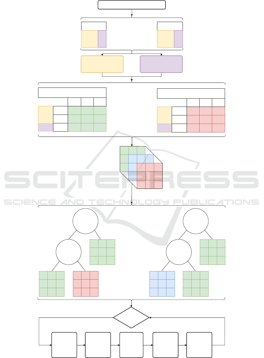
Firstly, we build a 3D matrix concatenating the
classifiers’ predictions in the following order: training
and testing. In this matrix, the first dimension repre-
sents the classifier, the second represents the sample
objects, and the third represents the class. Therefore,
each matrix cell represents the value predicted for a
specific category by a classifier for a given sample ob-
ject.
The second step concerns normalizing the 3D pre-
diction matrix using an initial function that places the
initial predictions in the range [0, 1]. We employed the
softmax function for this work, but other functions,
such as normalization and sigmoid, can be used.
In the third step, we start the optimization process.
The algorithm creates a random population of size
population size + new individuals. The random gen-
eration of each tree follows some restrictions: (i) the
root node is always a function (calculation) node, (ii)
the node with a depth equal to max depth is always an
extraction node, and (iii) the remaining nodes are cho-
sen randomly between the calculation functions and
the extraction function.
It is important to note that the relationship be-
tween population size and the number of genera-
tions is inversely proportional. A larger population
may require fewer generations to find optimal solu-
tions, and vice versa. In addition, the available GPU
memory capacity plays a crucial role in determin-
ing the population size. A higher GPU capacity al-
lows for larger populations, making exploring the so-
lution space more comprehensively in fewer genera-
tions easier.
Once the population is generated, each tree’s qual-
ity is calculated, which is the accuracy in the training
set of the prediction matrix resulting from the tree.
Then, the algorithm performs the crossover operator
based on each tree’s fitness and applies the mutation
operator to each resulting tree. Furthermore, new ran-
dom individuals are generated (new individuals) and
then added to the population. These processes repeat
until the number of generations is reached.
In this work, GP comprises two types of nodes:
• Prediction matrix extraction nodes: these nodes
are always leaves of the tree and copy one of the
2D matrices of some classifier. When generating
these nodes, a classifier is chosen randomly.
• Function nodes: when this type of node is gen-
erated, one of the functions is randomly chosen.
Table 1 lists all available functions employed in
this work.
Notice that this approach can be applied to any
classification problem, i.e., text, image, video, audio,
or a combination of classifiers designed for different
types of data, i.e., some video classifiers to classify
the video, while text classifiers to analyze and cate-
gorize the video description. The only requirement is
that the order of the sample objects and classes must
be the same in all classifiers.
Figure 1 illustrates the pipeline regarding the
methodology of this work.
3.1 Datasets
The experiments were performed on two datasets:
• The HMDB51 dataset is a large collection of re-
alistic videos from movies and web videos, com-
prising 6,766 clips in 51 action categories, with
a fixed frame rate of 30 FPS, a fixed height of
240, and a scaled width to maintain the original
aspect ratio. These categories cover a wide range
of human actions, like driving, fighting, running,
and drinking, among other classes (Kuehne et al.,
2011).
• The UCF101 dataset, an extension of UCF50,
contains 13,320 video clips classified into 101 cat-
egories. All videos are sourced from YouTube,
with a fixed frame rate of 25 FPS and a resolution
of 320×240. Some videos may include difficul-
ties like inadequate lighting, busy backgrounds,
and significant movement of the camera (Soomro
et al., 2012).
3.2 Experimental Setup
In this section, we present the experimental setup con-
cerning the optimization process employing the GP
algorithm:
• Maximum depth of the tree (max depth): [2, 7].
• Population size (population size): 20 and 10 for
HMDB51 and UCF101, respectively.
• New individuals (new individuals): 10 and 5 for
HMDB51 and UCF101, respectively.
• Number of generations: 400.
• Mutation rate (mutation rate): 0.5.
The values above were empirically set.
Six groups of functions are used in this work:
Mathematical, Fuzzy, Geometric, Average, Weighted
Average, and Self-Functions. All these functions ad-
here to a crucial premise: they accept input values
in the range [0, 1] and return values within the same
interval. The specific functions can be found in Ta-
ble 1. Weighted average and self-math functions are
the foundation for the system’s core functions, which
VISAPP 2024 - 19th International Conference on Computer Vision Theory and Applications
790

0.5
0.2
0.3
0.7
0.2
0.1
0.1
0.5
0.4
0.1
0.8
0.1
0.6
0.2
0.2
0.3
0.3
0.4
Concatened Train and Test set prediction matrix
of pre-trained classifier 1
0.5
0.2
0.3
0.7
0.2
0.1
0.1
0.5
0.4
0.3
0.4
0.3
0.2
0.7
0.1
0.8
0.2
0
0.1
0.8
0.1
0.6
0.2
0.2
0.3
0.3
0.4
Classifiers
Samples
Classes
Math multiply
Harmonic
average
0.5
0.2
0.3
0.7
0.2
0.1
0.1
0.5
0.4
0.5
0.2
0.3
0.7
0.2
0.1
0.1
0.5
0.4
0.1
0.8
0.1
0.6
0.2
0.2
0.3
0.3
0.4
Fuzzy Einstein
Sum
Fuzzy
Implication
0.5
0.2
0.3
0.7
0.2
0.1
0.1
0.5
0.4
0.5
0.2
0.3
0.7
0.2
0.1
0.1
0.5
0.4
...
No
Stop criterion is met?
0.3
0.4
0.3
0.2
0.7
0.1
0.8
0.2
0
Calculate the
fitness for each
tree
Crossover Mutation
Generate new
random
individuals and
add them to the
population
Save M best
individuals in a
file
Generate Initial Population
Concatened Train and Test set prediction matrix
of pre-trained classifier N
Dataset
Split 1
Train
Test
Split N
Train
Test
...
Train set
Samples that at last one
classifier saw in previus
training phase
Test set
Samples that no classifier
saw in previus training phase
Train set
Test set
Train set
Test set
Class 1
Class 2
Class 3
Sample 1
Sample 2
Sample 3
Class 1
Class 2
Class 3
Sample 1
Sample 2
Sample 3
...
Figure 1: Pipeline regarding the entire methodology employed in this work.
Strategies for Classifier Selection Based on Genetic Programming for Multimedia Data Recognition
791

utilize metrics for their operations. Available metric
functions in the system include accuracy, F1-score,
precision score, recall score, Jaccard score, and their
inverses (1 - metric). There are 41 pure functions, six
base functions, five metrics, and five inverse metrics.
The GP algorithm ensures that all generated indi-
viduals or solutions are valid. This is accomplished
using functions with inputs and outputs within the
range of 0 to 1, as outlined in Table1. Randomly se-
lecting these functions during node creation is a cru-
cial algorithm aspect, promoting solution diversity.
This method eliminates the possibility of generating
invalid individuals, ensuring the consistency and va-
lidity of the classifier combinations throughout the
process.
4 EXPERIMENTAL RESULTS
This section delves into the comprehensive experi-
mental analysis conducted using the HMDB51 and
UCF101 datasets. Employing advanced classifiers
and GP, the experiments aim to explore and enhance
the capabilities of our algorithm. The findings from
these experiments offer valuable insights into the ef-
fectiveness of GP in optimizing classifier committees,
showcasing the potential of these methods in machine
learning.
4.1 Classifiers
The classifiers used in this study were the ones used
by Santos and Almeida (2020), as follows:
• MV Classifier: it uses Motion Vectors (MV) for
video classification. The ResNet-18 architecture
focuses on capturing and analyzing motion varia-
tions between consecutive frames. In this context,
MV serves as a means to highlight dynamic dif-
ferences and changes across frames, essential for
efficient video compression and for recognizing
motion patterns (Santos and Almeida, 2020).
• DCT Classifier: it employs the Discrete Cosine
Transform to classify videos in the ResNet-50 ar-
chitecture. This approach uses DCT to convert vi-
sual information from n-frames into a frequency
representation. This conversion enables more ef-
ficient identification of important visual features
for video compression and analysis, making DCT
an effective method for processing large volumes
of visual data and reducing them to essential com-
ponents for classification (Santos and Almeida,
2020).
• DCT w/ FBS (DCT with Frequency Band Se-
lection) 16 and 32 classifiers: they represent ad-
vanced variations of the ResNet-50 architecture,
adapted to include the Frequency Band Selec-
tion (FBS) technique. FBS is used to select the
most relevant DCT coefficients in each n-frames.
The variants ”DCT w/ FBS 16” and ”DCT w/ FBS
32” differ in the number of DCT coefficients pro-
cessed per color channel. These approaches are
designed for more accurate and efficient analysis
of compressed video data, focusing on optimizing
action recognition in videos (Santos and Almeida,
2020).
4.2 HMDB51
This section presents the experimental results ob-
tained using the 12 trained classifiers provided by
Santos and Almeida (2020). The classifiers were
trained on three splits created by randomly selecting
videos from the complete HMDB51 dataset, denoted
as D. Each split consists of its own training and test-
ing subsets, denoted as D
train
i
and D
test
i
, respectively,
for (i = 1, 2, 3).
To evaluate GP in ensemble pruning, we defined
a new training set as the union of the training subsets
from all three splits, D
GPTrain
= D
train
1
∪D
train
2
∪D
train
3
,
which accounts for approximately 90% of the en-
tire HMDB51 dataset. The new test set, D
GPTest
,
comprises the elements in D that are not present
in D
GPTrain
, formally represented as D
GPTest
= D −
D
GPTrain
, constituting the remaining 10% of the
dataset.
Table 2 shows the accuracy of each classifier on
these new sets, as well as the best result obtained by
the GP algorithm, highlighted in bold. The GP algo-
rithm was executed at different depths (2 to 7), con-
sidering the fitness function as the training accuracy.
The best three results obtained in each depth are pre-
sented in Table 4 (see Section 5).
The results demonstrate the algorithm’s effective-
ness in the context of the HMDB51 dataset, as de-
tailed in Table4. The table outlines the accuracy of
each classifier across different training and testing
splits. This provides insights into the adaptability and
efficiency of our GP approach in dealing with varied
data characteristics, showcasing its ability to enhance
classification accuracy significantly.
4.3 UCF101
Similar to Section 4.2, this section details the ex-
perimental results obtained using classifiers on the
UCF101 dataset. For this experiment, we em-
VISAPP 2024 - 19th International Conference on Computer Vision Theory and Applications
792

Table 1: List of functions.
Math Geometric
Name Function Name Function
mult x ×y tanh
tanh(x)+1
2
Fuzzy circular
p
clamp(1 −x
2
, 0, 1)
Name Function elliptical
p
clamp(1 −x
2
−y
2
, 0, 1)
or max(x, y) parabolic clamp(1 −x
2
, 0, 1)
nor 1 −max(x,y) sine
sin(x)+1
2
and min(x, y) cosine
cos(x)+1
2
nand 1 −min(x,y) sigmoid
1
1+exp(−10×(x−0.5))
not 1 −x Average
xor abs(x −y) Name Function
xnor 1 −abs(x −y) average
x+y
2
implication min(1 −x,y) average geometrical
√
x ×y
concentration x
2
average harmonic
2
1
max(x,ε)
+
1
max(y,ε)
dilation
√
x average quadratic
q
x
2
+y
2
2
algebraic sum x + y −x ×y average cubic

x
3
+y
3
2

1
3
bounded sum min(x + y, 1) Weighted Average
bounded difference max(x −y, 0) Name Function
more or less 0.5 ×(
√
x + x) weighted average
x×wx+y×wy
max(wx+wy,ε)
implication godel 1 if x ≤ y else y weighted geometrical (
√
x
wx
×y
wy
)
1
max(wx+wy,ε)
implication lukasiewicz min(1,1 −x + y) weighted harmonic
wx+wy
wx
max(x,ε)
+
wy
max(y,ε)
einstein sum
x+y
1+x×y
weighted quadratic
q
x
2
×wx+y
2
×wy
max(wx+wy,ε)
einstein product
x×y
2−(x+y−x×y)
weighted cubic

x
3
×wx+y
3
×wy
max(wx+wy,ε)

1
3
negation yager
√
1 −x
2
Self Math
implication mamdani min(x, y) Name Function
implication zadeh max(1 −x, min(x, y)) self mult x × f (x)
gamma operator (x
z
×y
z
)
1
z
implication goguen min

y
x
, 1

if x > 0 else 1
clamped hamacher sum
x+y−2×x×y
max(1−x×y,1e−6)
hamacher product clamp

x×y
max(x+y−x×y,1e−6)
, 0, 1

exponential exp(−(1 −x)
2
)
logistic
1
1+exp(−x)
sigmoidal contrast
1
1+exp(−z×(x−y))
ployed all four classifiers from the first split of the
UCF101 dataset, denoted as Split 1. The training set,
D
UCFTrain
, was defined as the training subset of Split
1, D
train
1
. The test set, D
UCFTest
, was built by subtract-
ing the training set from the entire UCF101 dataset,
represented as D
UCFTest
= D
UCF
−D
UCFTrain
. This
approach was necessary because including an addi-
tional split would have resulted in all videos in the
database being seen by at least one classifier, poten-
tially skewing the research findings.
Table 3 presents the accuracy of each of the four
classifiers on these datasets. The result of the ensem-
ble pruning method using GP is highlighted in bold.
It is noteworthy that the GP algorithm was applied at
varying depths (2 to 7), with the accuracies in train-
ing, testing, and the combined value being detailed in
Table 5 at Section 5.
The findings of the UCF101 dataset, as detailed in
Table5, highlight the algorithm’s robustness. The ta-
ble displays the classifiers’ performance metrics, em-
phasizing the improved accuracy achieved through
our approach. This underscores the potential of GP
in optimizing classifier committees, even in scenarios
where initial classifier performance is already high.
Strategies for Classifier Selection Based on Genetic Programming for Multimedia Data Recognition
793

Table 2: Accuracy of the classifiers on the new subsets
based on work of Santos and Almeida (2020).
Split 1
Classifier name Train Test
MV 68,41% 29,43%
DCT w/ FBS (16) 69,18% 36,40%
DCT w/ FBS (32) 74,43% 37,10%
DCT 72,39% 36,82%
Split 2
Classifier name Train Test
MV 68,74% 32,78%
DCT w/ FBS (16) 70,90% 34,59%
DCT w/ FBS (32) 68,06% 26,78%
DCT 69,27% 37,24%
Split 3
Classifier name Train Test
MV 77,70% 26,50%
DCT w/ FBS (16) 64,69% 28,03%
DCT w/ FBS (32) 69,10% 33,33%
DCT 60,59% 22,59%
Ensemble
Classifier name Train Test
Ours 92.20% 45.23
Table 3: Accuracy of the 4 classifiers from split 1 on the new
subset of UCF101, based on work of Santos and Almeida
(2020).
Split 1
classifier name Train Test
MV 97.53% 73.86%
DCT w/ FBS (16) 99.90% 76.84%
DCT w/ FBS (32) 99.98% 78.77%
DCT 99.97% 77.37%
Ensemble
classifier name Train Test
Ours 100.00% 80.60%
5 ABLATION
Tables 4 and 5 present the full ablation results for the
HMDB51 and UCF101 datasets, respectively. These
results were obtained by executing the GP algorithm
at different depths (ranging from 2 to 7).
6 DISCUSSION
One may observe that GP is adept at identifying new
functions to combine committee members’ predic-
tions, although this can sometimes lead to reduced
performance in others, akin to overfitting. Notably,
Table 4: Top three trees by maximum tree depth in
HMDB51 dataset considering 16 classifiers.
Depth 2
Rank Train Test Sum
1 88.32% 41.08% 129.40%
2 39.15% 53.48% 92.43%
3 88.32% 41.08% 129.40%
Depth 3
Rank Train Test Sum
1 90.87% 45.57% 136.45%
2 41.17% 63.00% 110.18%
3 82.92% 54.57% 137.49%
Depth 4
Rank Train Test Sum
1 92.20% 45.23% 137.43%
2 50.32% 66.19% 116.51%
3 89.80% 48.92% 138.72%
Depth 5
Rank Train Test Sum
1 91.46% 41.50% 132.96%
2 46.46% 65.00% 111.46%
3 87.89% 50.67% 138.56%
Depth 6
Rank Train Test Sum
1 91.98% 43.35% 135.33%
2 47.81% 66.69% 114.50%
3 91.05% 46.98% 138.02%
Depth 7
Rank Train Test Sum
1 90.70% 38.01% 128.71%
2 49.57% 63.46% 113.04%
3 86.06% 58.59% 144.65%
there are instances where GP-derived functions en-
hance performance across both training and test sets
simultaneously, indicating a nuanced understanding
of the data characteristics.
A case in point is the result at depth 7 in the
HMDB51 dataset, where we witnessed an increase of
9% of accuracy in the training set and a significant in-
crease of 20% of accuracy in the test set considering
the best individual classifier exemplifying the versa-
tility of GP as a tool. It enables users to tailor the
function to their specific requirements, whether prior-
itizing training set accuracy, test set accuracy, or seek-
ing a balance between the two.
In the UCF101 dataset, we encountered a different
challenge. The classifiers already demonstrated high
accuracy levels, achieving up to 99.96% of accuracy
for training and 83.20% of accuracy for testing, leav-
ing limited room for improvement. However, when
considering the tree depth of size 7, we witnessed a
remarkable instance of GP’s effectiveness in further
VISAPP 2024 - 19th International Conference on Computer Vision Theory and Applications
794

Table 5: Top three trees by maximum tree depth in UCF101
dataset considering four classifiers.
Depth 2
Rank Train Test Sum
1 100.00% 79.79% 179.79%
2 99.56% 81.45% 181.01%
3 99.91% 81.36% 181.27%
Depth 3
Rank Train Test Sum
1 100.00% 79.79% 179.79%
2 99.99% 82.73% 182.72%
3 99.99% 82.73% 182.72%
Depth 4
Rank Train Test Sum
1 100.00% 80.30% 180.30%
2 99.99% 82.89% 182.88%
3 99.99% 82.89% 182.88%
Depth 5
Rank Train Test Sum
1 100.00% 80.77% 180.77%
2 99.96% 82.93% 182.89%
3 99.96% 82.93% 182.89%
Depth 6
Rank Train Test Sum
1 100.00% 79.14% 179.14%
2 99.98% 83.23% 183.21%
3 99.98% 83.23% 183.21%
Depth 7
Rank Train Test Sum
1 100.00% 80.66% 180.66%
2 99.96% 83.20% 183.16%
3 99.96% 83.20% 183.16%
optimizing these results. Despite a minimal loss of
0.4% in the training accuracy, there was a significant
gain of 4.43% of accuracy in the test set, highlighting
the GP’s capability to fine-tune classifier performance
even in scenarios where the improvement margin ap-
pears to be minimal.
The flexibility offered by GP, as demonstrated by
the varying performances at different depths (notably
depths 6 and 7), underscores its utility in diverse clas-
sification scenarios. One can use this adaptability to
fine-tune their models, achieving an optimal balance
between training and test performances that align with
their specific goals and constraints.
7 CONCLUSIONS
In conclusion, this study underscores the potential of
GP in ensemble pruning, particularly in optimizing
classifier selection and the function that will be used
to combine the predictions. Our findings reveal that
GP can effectively balance the performance between
training and test sets, offering a versatile tool for vari-
ous classification challenges. This work observed sig-
nificant improvements at various depths, especially
at depth 6, highlighting GP’s ability to adapt to data
characteristics and user requirements.
In future work, it would be intriguing to expand
the repertoire of functions used by the GP, potentially
uncovering even more effective combination methods
for classifiers. Additionally, experimenting with dif-
ferent types of classifiers beyond those used in this
study could provide deeper insights into the versatility
and efficacy of GP in various classification contexts.
Another significant direction is applying GP to
diverse data types, such as audio, images, text, and
video. Investigating how GP performs across these
different modalities could reveal unique challenges
and opportunities, further enhancing the understand-
ing of its adaptability and effectiveness. Testing GP
in these varied scenarios will broaden its applicabil-
ity and contribute to developing more robust and ver-
satile machine learning models capable of handling
complex, multi-modal datasets.
REFERENCES
Koza, J. R. (1992). Genetic Programming: On the Pro-
gramming of Computers by Means of Natural Selec-
tion. MIT Press, Cambridge, MA, USA.
Kuehne, H., Jhuang, H., Garrote, E., Poggio, T., and Serre,
T. (2011). HMDB: a large video database for human
motion recognition. In Proceedings of the Interna-
tional Conference on Computer Vision (ICCV).
Santos, S. F. and Almeida, J. (2020). Faster and accurate
compressed video action recognition straight from
the frequency domain. In 2020 33rd SIBGRAPI
Conference on Graphics, Patterns and Images (SIB-
GRAPI). IEEE.
Soomro, K., Zamir, A. R., and Shah, M. (2012). Ucf101: A
dataset of 101 human actions classes from videos in
the wild.
Statista (2023). Data growth worldwide 2010-2025.
https://www.statista.com/statistics/871513/
worldwide-data-created. Accessed: 2023-08-22.
Wu, C.-Y., Zaheer, M., Hu, H., Manmatha, R., Smola, A. J.,
and Kr
¨
ahenb
¨
uhl, P. (2018). Compressed video action
recognition.
Zhou, Z.-H. (2021). Machine learning. Springer Nature.
Strategies for Classifier Selection Based on Genetic Programming for Multimedia Data Recognition
795