Making Hard(er) Benchmark Functions:
Genetic Programming
Dante Niewenhuis
1 a
, Abdellah Salhi
2 b
and Daan van den Berg
1,3 c
1
Department of Computer Science, Vrije Universiteit Amsterdam, The Netherlands
2
Department of Mathematical Sciences, University of Essex, U.K.
3
Universiteit van Amsterdam, The Netherlands
Keywords:
Genetic Programming, Fitness Landscapes, Evolutionary Algorithms.
Abstract:
TreeEvolver, a genetic programming algorithm, is used to make continuous mathematical functions that give
rise to 3D landscapes. These are then empirically tested for hardness by a simple evolutionary algorithm, after
which TreeEvolver mutates the functions in an effort to increase the hardness of the corresponding landscapes.
Results are wildly diverse, but show that traditional continuous benchmark functions such as Branin, Easom
and Martin-Gaddy might not be hard at all, and much harder objective landscapes exist.
1 INTRODUCTION
Branin, Easom, Martin-Gaddy and the Six-Hump
Camel are household names in the evolutionary pro-
gramming community. Being strictly mathematically
formulated benchmark functions, they define con-
tinuous objective landscapes
1
with precisely known
global minima in both values and locations, and a di-
verse range of hardness features such as many local
minima, narrow basins or arctic plateaus on which
metaheuristic navigation is almost impossible.
As household names do, these benchmark func-
tions are well-known throughout the practicioner’s
field and are often used for testing and comparing
optimization algorithms such as simulated annealing,
genetic algorithms and ant colony optimization, but
also machine learning (Fodorean et al., 2012; Joshi
et al., 2021; Digalakis and Margaritis, 2001; Laguna
and Marti, 2005; Socha and Dorigo, 2008; Orze-
chowski and Moore, 2022). Though one could easily
mistake such reuse as intellectual poverty or just plain
trendy, experimenting on a limited set of benchmark
test functions actually has its upsides too, as it en-
ables papers to be tied together, percolating our grains
a
https://orcid.org/0000-0002-9114-1364
b
https://orcid.org/0000-0003-2433-2627
c
https://orcid.org/0000-0001-5060-3342
1
Please note that we deliberately omit the term “fit-
ness landscapes” as objective values and fitness values are
strictly spoken not interchangeable.
of knowledge to larger clusters of more or less uni-
versally true principles. Benchmarking is important.
So important even, that the study of ‘best practice’ in
benchmarking has become a focus of scientific study
in itself (Bartz-Beielstein et al., 2020).
Household names are individuals we are familiar
with, that have known properties, and show pre-
dictable behaviour. This is no different for continu-
ous or discrete optimization problem suites; the most
famous example of which is undoubtedly TSPLib,
Gerhard Reinelt’s library of traveling salesman prob-
lem instances (Reinelt, 1991). The traveling salesman
problem as a whole is NP-hard, meaning there is no
known polynomial-time exact algorithm, thereby ob-
structing a view on the shortest tour, even for mod-
erately sized instances. To make things worse, we
also don’t know its length. From this point, we have
to fight from the numerical jungle, using guerilla al-
gorithmics and tailor-made pattern hacks such as ex-
ploiting Euclideaness, bootstrapping upper bounds
or exploit undiverse numerical values (Sleegers and
van den Berg, 2020a; Koppenhol et al., 2022; Apple-
gate et al., 2009; Zhang and Korf, 1996). It is there-
fore not surprising that many TSP-instances only have
a best known solution instead of a best solution - a
phenomenon that occurs in many more combinatorial
optimization problems (Rosenberg et al., 2021; Weise
et al., 2021; Weise and Wu, 2018).
The situation is slightly different for continuous
problems. Here, our household benchmark functions
Niewenhuis, D., Salhi, A. and van den Berg, D.
Making Hard(er) Benchmark Functions: Genetic Programming.
DOI: 10.5220/0012475800003690
Paper published under CC license (CC BY-NC-ND 4.0)
In Proceedings of the 26th International Conference on Enterprise Information Systems (ICEIS 2024) - Volume 1, pages 567-578
ISBN: 978-989-758-692-7; ISSN: 2184-4992
Proceedings Copyright © 2024 by SCITEPRESS – Science and Technology Publications, Lda.
567

Figure 1: Some ‘household names’: continuous benchmark functions that are often used in testing evolutionary algorithm
performance. But how hard are these objective landscapes really? Do harder instances exist?
usually not only have known global minimum values,
but their exact location is also known, as are the land-
scape features. Sometimes these known properties
even extend to parameterizable higher dimensions, so
that even for a 257-dimensional Ackley function, the
global minimum value - and its location - is known.
Such scaleup is only dreamt of in TSP-communities,
where the addition of just a few cities to a known in-
stance can distort all its properties, except in the most
structured of cases, such as circular or grid instances.
Stop reading and contemplate this for a minute. Why
is the scaleup in discrete benchmarking so different
from the scaleup in continuous benchmarking? Why
is it so much harder to find minima for larger search
spaces in discrete problems as opposed their continu-
ous counterparts?
2
The answer, we will provisionally argue, is struc-
ture or the lack thereof, in the universalest sense of
the word. By an argument of Kolmogorov complex-
ity, easy traveling salesman instances are those whose
cities are placed on a circle, on a grid, or on the ver-
tices of a regular fractal (Fischer et al., 2005). These
are easy, and have known global minima, both in
value and location (or exact tour configuration) as
they scale up. Nonetheless the computer programs
needed to describe these instances remain relatively
small, and hence their Kolmogorov complexity is low.
In fact, an investigation by Fischer, St
¨
utzle, Hoos
and Merz showed that these regular instances become
2
Did you stop reading for a minute?
harder when the TSP instance’s city locations are dis-
torted. The greater the distortion, the less structured
the instance, the longer the algorithmic description,
and the higher the Kolmogorov complexity. In other
words: there is evidence that structured (or equiva-
lent: shortly describable) instances of TSP are eas-
ier than unstructured (or not shortly describable) in-
stances, which are harder to solve. And recently,
similar phenomenon has also appeared in the NP-
complete Hamiltonian cycle problem, where only the
extremely hard and extremely easy instances appear
to be highly structured (Sleegers and van den Berg,
2020a; Sleegers and van den Berg, 2020b; Sleegers
and Berg, 2021; Sleegers and van den Berg, 2022).
Moreover, these studies also suggests that the break-
down of an instance’s structure influences its hard-
ness, even though this specific case pertains to a deci-
sion problem.
Now, the key question is of course: to what ex-
tent can the same argument apply to continuous opti-
mization? Are continuous landscapes with structure,
with short descriptions, with low Kolmogorov com-
plexity also easier than those with without structure,
or long descriptions? They might. There is some ev-
idence that the hardness of several continuous bench-
mark functions such as Schwefel, Rastrigin and Ack-
ley decreases with increasing numbers of dimensions
(De Jonge and Van den Berg, 2020; de Jonge and
van den Berg, 2020). This shoehornily fits our pro-
visional hypothesis because these functions usually
increase their dimensionality (and thereby the search
ICEIS 2024 - 26th International Conference on Enterprise Information Systems
568

Figure 2: Example of different function trees. Functions are green, operators red and both variables and constants are grey.
space) by upping the D-parameter in its main term,
which usually looks like
∑
D
d=1
F(x
d
). In other words:
the functional description (or Kolmogorov complex-
ity) remains short, and does not increase along with
the search space, much like an highly regular TSP-
instance.
We’ll skip the quite interesting question of why
these benchmarks are the way they are for now, but
rather ask: could they have been different? Could
substantially different hard objective landscapes ex-
ist, and what do they look like? The answer is yes,
and we can find out by evolving the tree structure of
the objective functions (Fig. 2). This concept, the
evolutionarily improvement of computer programs, is
known as genetic programming and was introduced
by John Koza in “Genetic Programming On the Pro-
gramming of Computers by Means of Natural Selec-
tion” (Koza, 1992; Koza, 1994). Whereas genetic al-
gorithms operate on strings, numbers or data struc-
tures, genetic programming evolves the source code
itself (Sette and Boullart, 2001). It has been applied
to a large number of problems such as robotics (Koza
and Rice, 1992), financial modelling (Kordon, 2010),
image processing (Lam and Ciesielski, 2004), and de-
sign (Koza, 2008). In artificial intelligence genetic
programming has been used for tasks such associated
discovery (Lyman and Lewandowski, 2005) and clus-
tering (Alhajj and Kaya, 2008; Bezdek et al., 1994;
De Falco et al., 2006; Jie et al., 2004; Liu et al.,
2005). One survey notably provides an overview of
more than 100 applications of genetic programming
(Espejo et al., 2009).
In this work, we’ll take a somewhat more con-
servative approach than abovementioned examples,
“just” evolving the objective functions giving rise to
the corresponding three-dimensional landscapes. As
such, an easy-to-minimize function like x
1
+x
2
might
evolve to something like (−1.203 − 10) ∗ 1.855 +
sin(x
2
+6.363−x
1
)+sin(−0.197+x
2
), which is very
hard to minimize for an evolutionary algorithm. The
task is therefore formulated as ‘make a hard objective
landscape’, (for some evolutionary algorithm). More
generally however, it is the beginning of an explo-
ration into the combinatorial space of continuous ob-
jective landscapes. We, the community, are all too fa-
miliar with our household names like Mishra, Easom
and Goldstein-Price ... but what else is out there?
2 OBJECTIVE LANDSCAPE
HARDNESS
Evolving objective landscapes for hardness requires
measuring that hardness. In evolutionary computing,
a popular performance metric is the mean best fit-
ness (MBF) (Eiben et al., 2003), which averages the
best results from a number of runs on an objective
landscape. While suitable for the comparison two al-
gorithms, we rather require a method that compares
the performance of two landscapes. In other words:
is algorithm
1
more succesful on objective landscape
OL
1
or on objective landscape OL
2
? For such an as-
sessment, the MBF is unsuitable because a better end
result on OL
2
means nothing if OL
2
’s global mini-
mum value is much lower, or the individuals get ini-
tialized much higher.
In a variation on MBF therefore, we will measure
the performance of an evolutionary run relative to an
objective landscape’s global minimum, denoted as its
objective deficiency (Niewenhuis and van den Berg,
2022; Niewenhuis and van den Berg, 2023):
v −OL
min
OL
max
−OL
min
∗100 (1)
in which OL is an objective landscape and OL
min
and
OL
max
are the values of the global minimum and max-
imum respectively. The range of a benchmark is de-
Making Hard(er) Benchmark Functions: Genetic Programming
569

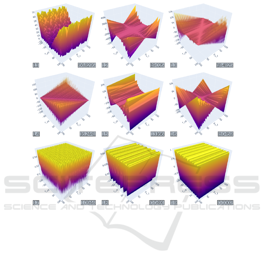
Figure 3: Objective landscapes from experiment 1 after 2000 generations in TreeEvolver, ordered by MOD. All runs had
x
1
+ x
2
as their initial function. Operator nodes were limited to {+, −,∗}, and Function nodes were limited to {sin}.
fined as the difference between OL
min
and OL
max
and
v is an assessable value, for instance ‘the best individ-
ual of an EA after 2000 evaluations’. When averag-
ing over several (stochastic) runs, we obtain the Mean
Objective Deficiency (MOD). In this work we consis-
tently do 100 runs of the Plant Propagation Algorithm
(PPA) (Section 3) for every MOD-assessment.
There is still a problem however. Whereas house-
hold benchmark functions such as Ackley, Goldstein-
Price and Six-Hump Camel have precisely known
global minima and can therefore easily be assessed,
this is no longer the case for evolved objective land-
scapes. And finding them is also not easy; a preli-
mary run showed that calculating zero-derivatives of
evolved objective landscapes, a conceptually ideal ap-
proach, is computationally infeasible, unreliable and
in some cases even impossible from the incorpora-
tion of absolute signs, divisions by zero, square roots
and logarithms. For that reason, after every mutation
(’generation’) we obtained a surrogate global maxi-
mum and minimum from 10
6
random objective sam-
ples from the evolved function’s domain. This method
works well for getting the concept working, but more
sophisticated future methods, or tighter restrictions on
the mutation types are definitely not unthinkable.
For sakes of comparison, we also assessed
the MOD of the household names from Fig-
ure 1. Sorted from hard to easy: MOD
Easom
=
14.26, MOD
Mishra04
= 0.925 MOD
Branin
= 2.297e −
04, MOD
SixHump
= 7.149e −04, MOD
MartinGaddy
=
3.077e −04 and MOD
GoldsteinPrice
= 1.831e −05 . It
seems safe to conclude that only Easom is slightly
hard for PPA; the rest are easy.
3 THE PLANT PROPAGATION
ALGORITHM
Before we come to the evolutionary algorithm of
choice, let’s start with a few substantial disclaimers.
We, the authors, are fully aware of the massive debate
ICEIS 2024 - 26th International Conference on Enterprise Information Systems
570

Table 1: The 9 objective from experiment 1 ordered by MOD. All runs had x +y as their initial function. Operator nodes were
limited to {−,+, ∗}, and Function nodes were limited to a value from {sin}.
MOD Function
1.1 66.8295
(sin(9.483 ∗(sin(x
2
) +x
1
)) ∗x
2
+ x
2
) ∗sin(9.341 ∗5.656 ∗(x
1
+ sin(x
1
)) ∗x
2
∗x
2
∗
x
2
∗x
1
∗(x
1
−x
2
∗x
2
−2.198 + x
2
−x
2
+ sin(x
2
) ∗2.775 ∗x
2
))
1.2 19.0250
x
1
∗((sin(−2.289)+ 5.171) ∗5.299 −x
2
∗x
2
−x
2
+ 5.102)∗(sin(sin(sin(sin(−1.105)))∗
sin(−4.52 ∗(sin(sin(3.104)) −sin(sin(sin(sin(sin(−6.796 −3.117 ∗8.209) + sin(sin(x
2
+x
2
) +x
2
)))))))) −sin(−3.105))
1.3 18.4825
(sin(sin(9.882)) + (sin(x
1
+ 10)+ sin(6.877)) ∗(x
2
−x
1
) ∗sin(sin(−6.488) −4.68∗
sin(x
2
) +x
2
) ∗sin(x
2
) ∗x
2
) ∗sin(x
2
+ x
2
∗(x
2
−sin(x
2
)))
1.4 16.2441
(x
2
+ x
1
) ∗(sin(−1.689 + 1.36)+ sin(sin(4.549) +sin(sin(sin(sin(x
2
) −1.991)))+
sin(−8.193 +3.761 ∗(−8.649 −sin(sin(sin(sin(x
2
−sin(2.983)−sin(sin(x
1
−9.285−
sin(sin(sin(x
1
+ 9.01)))))))))))+ x
2
)) ∗sin(x
2
)
1.5 13.1660
(2.792 +(−8.546 + x
2
−sin(sin(sin(sin(sin(sin(sin(sin(−10 ∗x
2
)))))))) ∗sin(0.383) ∗(
x
2
+ x
1
) −10) ∗sin((10 + sin(sin(−5.099 +1.037 + sin(x
2
) +7.607))) ∗x
2
)) ∗(x
2
+ x
2
)
1.6 8.0459
(−10 −x
2
) ∗sin(x
1
+ x
1
−7.896 −sin(sin(sin(−8.594 −sin(1.416 ∗x
1
))) −9.702)) ∗(x
1
+6.539)
1.7 1.0944
sin(sin(sin(sin(sin(sin(sin(7.465 + sin(sin(−3.419 −x
2
) −4.721 + sin(x
1
+ x
2
)))))))))
1.8 0.0491
sin(sin(−5.657 +sin(sin(sin(sin(sin(sin(sin(sin(sin(x
2
−8.376)+ 7.648))) ∗2.174))))
−7.109)))
1.9 0.0002
sin(x
1
+ x
2
−7.345 −x
1
)
that has been unfolding in the community pertaining
to ‘metaphorical’ or ‘new’ evolutionary algorithms.
We would therefore like to clearly state that: the plant
propagation algorithm (PPA) is not newly introduced
here, its name is just a name and nothing more, and it
is not claimed to be competitive in any way. Reasons
to choose this algorithm is that we find it elegant, es-
pecially in self-balancing itsexploration and exploita-
tion, its easiness of implementation, availability of
open source and finally, because a lot is known about
its behaviour, also in different parameterizations, on
continuous objective landscapes (Fraga, 2019; Rod-
man et al., 2018; Sleegers and van den Berg, 2020a;
Sleegers and van den Berg, 2020b; Sulaiman et al.,
2018; Vrielink and van den Berg, 2019; Vrielink and
Van den Berg, 2021b; Vrielink and Van den Berg,
2021a; Geleijn et al., 2019; Haddadi, 2020; Paauw
and Berg, 2019; Selamo
˘
glu and Salhi, 2016; Su-
laiman et al., 2016). However, this GP-method is
not confined to PPA; other evolutionary algorithms or
perhaps even exact methods could also do the assess-
ment.
The central idea of PPA is idea that better indi-
viduals in its population produce more offspring with
smaller mutations while worse individuals produce
fewer offspring with larger mutations. Since fitness
values are normalized ∈ [0,1], the algorithm con-
stantly maintains a homeostatic balance between ex-
ploration and exploitation throughout its evolutionary
run. In other words: no matter how near or far the
population is from a global or local optimum, and no
matter what its population looks like, it will always
simultaneously keep exploiting and exploring. In this
work we are using the seminal implementation (in-
cluding parameter settings) as introduced by Salhi &
Fraga in 2011 (Salhi and Fraga, 2011), which goes
through the following steps:
1. Initialize a population of popSize=30 individuals
by sampling from a uniform distribution within in
the objective function’s domain.
2. Calculate the objective value f (x
i
) for each indi-
vidual in the current population.
3. Normalize the objective value f (x
i
) between 0
and 1 using z(x
i
) =
f
max
− f (x
i
)
f
max
− f
min
wherein f
min
and
f
max
are the lowest and highest objective values in
the current population.
4. Determine the fitness of each individual using
F(x
i
) =
1
2
(tanh(4 ∗z(x
i
) −2) + 1).
5. Determine the number of offspring for each indi-
vidual using n(x
i
) = ⌈n
max
F(x
i
)r
1
⌉, in which r
1
is a random number in [0, 1) and n
max
= 5 is the
parameter for the maximum number of offspring
from any individual.
6. Create the offspring of each individual by mutat-
ing each dimension j using (b
j
−a
j
)d
j
, in which
b
j
and a
j
are the upper and lower of dimension
j, and d
j
= 2(r
2
−0.5)(1 −F(x
i
)); r
2
is a random
number in [0,1).
7. Add all the offspring to the current population and
select the popSize individuals with the highest fit-
ness to become the next population.
8. If the number of function evaluations does not yet
exceed 5000, return to step 2.
Making Hard(er) Benchmark Functions: Genetic Programming
571

Table 2: TreeEvolver’s available function nodes and operator nodes for all 9 experiments in this paper. A diverse set of
initial conditions was used to explore the space of possibilities.
Exp Initial Functions Operators
1 x
1
+ x
2
sin -, +, *
2 x
1
∗x
2
+ 7 sin -, +, *
3 sin(x
1
) +sin(x
2
) sin -, +, *
4 x
1
+ x
2
sin −,+,∗,/,
∧
5 (x
1
/3) ∗(x
2
/6) sin −,+,∗,/,
∧
6 sin(x
1
)/5 +x
2
2
sin −,+,∗,/,
∧
7 x
1
+ x
2
sin, cos, sqrt, exp, abs -, +, *
8
√
x
1
∗|sin(x
2
)| sin, cos, sqrt, exp, abs -, +, *
9 cos(x
1
) ∗exp(x
2
) sin, cos, sqrt, exp, abs -, +, *
4 OBJECTIVE LANDSCAPES
FROM OBJECTIVE FUNCTION
TREES
In genetic programming, the most common represen-
tation of an evolvable program is a tree data structure
(Banzhaf et al., 1998). For continuous objective func-
tions such as in this study, this need not be different.
The binary trees representing the functions consist of
maximally four node types:
1. The single-child functions nodes con-
tain sin(x), cos(x), exp(x), abs(x) or
sqrt(abs(x)). Note that the abs inside the
sqrt is to accommodate consistency in the real
numbers, and avoid squarerrooting a negative
number.
2. The five operator nodes +, -, *, \ and ˆ all
have two child nodes left and right which
are processed inorder to accommodate for the
three non-commutative (or ‘asymmetric’) opera-
tors. As such, substraction is therefore under-
stood as left −right, division as left\right
and power as left
right
.
3. Variable nodes contain all occurrences of x
1
and
x
2
, given the fact that this study is limited to
two-dimensional objective functions (with three-
dimensional landscapes).
4. Constant nodes contain constant numeric values,
such as 6, −4.22 or −0.00004. The value of a
constant is kept within by the lowest power of 10
that encapsulates the initial value. For instance, if
a constant node is instantiated with the value 4.6,
its bounds will be [−10,10]. If a constant node
is instantiated with the value 3728 it will have the
bounds [−10.000,10.000].
A few examples of function trees can be seen in Fig-
ure 2. Note that it is possible for functions to be rep-
resented by different trees; for example x
1
+ x
2
+ 5
can have the first + or the second + as its root. In
such cases the first operator is designated the root
node. Furthermore, mathematical equivalents such
as (x
1
∗x
1
) versus (x
1
)
2
, which could be regarded
as symmetry in TreeEvolvers search space, is unad-
dressed.
5 EVOLVING OBJECTIVE
FUNCTION TREES
The TreeEvolver is an implementation of genetic
programming and follows a simple hillClimber
paradigm: it makes a single mutation to the func-
tion tree, assesses its new MOD-hardness, keeps the
new tree iff harder, and otherwise reverts the muta-
tion. Abiding by the well-known KISS-doctrine
3
, it
functions pretty well for getting the concept working,
but more sophisticated methods, such as population-
based tree evolvers, could certainly be incorporated
in future experiments – most notably because the
crossover operator can be readily implemented on this
concept. In the current implementation, the algorithm
begins each generation by creating a list of all eligible
mutations on the current function tree.
The first and most straightforward mutation type,
change node, is the only mutation type that does not
change the number of nodes in a function tree. For
trees to remain valid, the value of a selected node
can only be changed into a value of the same type,
e.g., a function node can only be changed into another
function node, and not into an operator node. For ex-
ample, a change from −4.27 to 5.5, a change from
sin(2 ∗x
1
+ 4) to exp(2 ∗x
1
+ 4) or a change from
exp(2 ∗ x
1
+ 4) to exp(
2
x
1
+ 4) are all valid change
3
Keep It Simple,Scientist!
ICEIS 2024 - 26th International Conference on Enterprise Information Systems
572

Figure 4: All 9 objective landscapes from experiment 5 after 2000 generations in TreeEvolver, ordered by MOD. All runs had
x
1
+ x
2
as their initial function. Operator nodes were limited to a value from [+, −,∗], and function nodes were limited to a
value from {sin}.
node mutations. If there is only one possible value for
a node type, and therefore the mutation would cause
no real change, it is not added to the list.
Second, insert function node creates a new ran-
dom functions node F, and then randomly chooses
an existing node N from the tree above which F is in-
serted. Changing 2 ∗x
1
−4∗x
2
to 2∗x
1
−cos(4∗x
2
) is
a valid insert function node mutation, and so is chang-
ing 2 ∗x
1
−4 ∗x
2
to |2 ∗x
1
−4 ∗x
2
|.
The third mutation type, remove function node,
randomly chooses a function node F from the current
tree at random, removes it, and links its child to its
parent. This mutation type will only be added to the
list when the function tree has at least one function
node.
Fourth, insert operator node first chooses a node
N in the current tree above which to insert a newly
randomly generated operator node O. Node N will
become one of O’s children, the other will be a ran-
domly generated variable node or constant node. Both
the choice variable-or-constant and the choice left-or-
right are made at random.
Fifth, remove operator node selects an existing
operator node from the tree, choosing one of its chil-
dren at random to take its place. The other of the two
children is deleted.
After listing all eligible mutations, a tree of n
nodes of which l leave nodes, the list will contain
4n −l mutations: n change node mutations, n insert
function node mutations, n insert operator node mu-
tations, n −l combined remove node mutations. A
mutation is then randomly chosen from the list of pos-
sibilities and executed on the given tree. Finally, a
check is performed whether the tree still holds at least
one of the variables x
1
or x
2
in at least one place,
which could have been accidentally deleted from a
subtree. If this is not the case, the mutation is reverted
and a different mutation is chosen.
Making Hard(er) Benchmark Functions: Genetic Programming
573

Table 3: The 9 objective from experiment 5 ordered by MOD. All runs had (x
1
/3) ∗(x
2
/6) as their initial function. Operator
nodes were limited to {−,+, ∗,/,
∧
}, and Function nodes were limited to a value from {sin}.
MOD Function
5.1 99.9978
(x
2
−sin(sin(4.572 ∗sin(sin(x
2
+ sin(sin(x
1
)) + 7.655/(3 + x
2
))))))
∧
sin(sin(sin(x
∧
1
(−2.454 ∗2.968))/x
2
/8.654)
∧
9.814)
5.2 99.9775
−6.199/x
∧
2
sin(sin(x
1
/sin(sin(sin(sin(sin(sin(sin(sin(sin(sin(x
1
)))/sin(−5.354))))))
∗sin(−1.081)))))
5.3 99.9433
sin(6.786/sin(sin(sin(sin(4.276))))/sin(−1.864))/(x
1
−4.944 + x
2
) ∗6
5.4 99.8452
x
2
/(sin(7.872) +7.652 ∗x
2
∗x
1
)
5.5 99.7811
−1.811/x
2
/x
2
∗1.817/7.001/(x
1
+ 9.93/sin(sin(x
2
))/x
1
)
5.6 99.7678
x
1
+ 2.447/x
1
/3 ∗3.563/sin(sin(−1.598))
5.7 99.7543
−2.373
∧
((−6.394 −x
1
)/x
1
/sin((3.648/4.956)
∧
2.674))/10 ∗sin(x
1
−6.537)/
sin(sin(6 −0.648
∧
−7.139))
5.8 98.7259
sin(sin(sin(sin(−4.426) ∗x
2
/7.683
∧
(sin(x
2
)/sin(x
1
)/sin(sin(sin(sin(3))))))))
x
1
/x
1
/sin(x
1
+ 10)
5.9 96.7829
sin(sin(sin(sin(sin(sin(sin(−6.487 +x
1
∗−0.244))
∧
sin(sin(sin(sin(sin(sin(x
2
))+
5.185)))/10))))))
6 EXPERIMENT & RESULTS
For this first exploration we conduct 9 experiments
with widely different combinations of available func-
tion nodes, operator nodes and initial objective func-
tions with a domain of [−100,100]
2
. Each initial
objective function will undergo 9 independent evolu-
tionary runs of 2000 generations in TreeEvolver, mak-
ing for a total of 81 runs. Exact settings of the exper-
iments can be found in Table 2, and full results are
publicly available (Anonymous, 2022). For this ex-
ploration, we will be discussing experiments 1, 5 and
8 as a representative overview of the enormous diver-
sity in results.
All experiments were run on a HP ZBook G5 with
Intel Core I7-750H processor and 16 GB RAM run-
ning Ubuntu 20.04.2 LTS. All Python code was writ-
ten in Python 3.10. All benchmark calculations are
done using NumPy 1.21.4. Analysis is done using
Pandas 1.3.4. Finally, Visualization of the bench-
marks is done using Plotly 5.4. For consistency,
all values are rounded to 10 decimals, and clipped
at −1,000, 000 and 1,000,000. All initial objective
functions have MOD = 0, and are thus extremely
easy.
6.1 Experiment 1
Experiment 1, the smallest in the ensemble, starts off
initial objective function x
1
+ x
2
, with operator nodes
∈ {+, −,∗} and function nodes ∈ {sin} available to
TreeEvolver. Table 1 holds the evolved functions af-
ter 2000 generations of the TreeEvolver in descending
MOD, while Figure 3 shows the corresponding objec-
tive landscapes.
Roughly speaking, we can divide the functions
into three groups. The first group consist solely of
1.1, a function that holds many multiplications and
significantly harder than all others in this ensem-
ble. Its landscape also looks quite a bit different.
The second group consist of the five functions that
are considerably less hard (1.2 to 1.6). Here, func-
tions have grown substantially larger and have nested
sin functions, and have ‘butterflyish’ shapes, some-
times even ‘hairy’. These recurring patterns might
tell us something about the hardness of these func-
tions, or the preferred evolutionary paths of TreeE-
volver. Finally, the existence of a group of easy func-
tions (1.7 −1.9) might signal that the intitial condi-
tions not optimally suited for making hard objective
functions. Of these nine results, the first five functions
are all substantially harder than our hardest house-
hold name, which is Easom with MOD
Easom
= 14.26,
which would come in fifth place here.
6.2 Experiment 5
Experiment 5, starting off from x
1
/3 + x
2
/6, hav-
ing operators ∈ {+,−,∗,/,
∧
} and function nodes ∈
sin}, resulted in some very hard objective landscapes
after 2000 generations in TreeEvolver. The func-
tional descriptions again show many nested sine func-
tions (Table 3), but the landscapes are very different
from experiment 1.1 (Figure 4). Instead of ‘hairy but-
terflies’, we now see largely flat stretches interrupted
by very narrow extremities, possibly caused by the di-
vision operator. Of these, 5.6 could be argued to be a
variation to the theme, as its tilt gives rise to a massive
deceptive basin, covering half its domain.
Completely different are 5.2, 5.8, and 5.9 which
ICEIS 2024 - 26th International Conference on Enterprise Information Systems
574

Figure 5: The 9 objective landscapes from experiment 9 after 2000 generations in TreeEvolver, ordered by MOD. All runs
had
√
x
1
∗|sin(x
2
)| as their initial function, operator nodes were limited to {−,+, ∗}, and Function nodes were limited to a
value from {sin,cos, sqrt,exp,abs}.
have large numbers of nested sin functions and
thereby have more of a ‘harmonicose structure’.
Nonetheless, with the lowest MOD = 96.78, these
functions are all very hard to minimize for PPA, and
demonstrate that there is definitely more than one way
of making hard objectives functions, and also that our
rather unsophisticated TreeEvolver can readily find
them in this experimental setting.
6.3 Experiment 8
TreeEvolver’s evolutionary trajectory from initial ob-
jective function sqrt(|(x
1
)|) ·|(sin(x
2
)|, with avail-
able operators ∈ {+, −,∗} and function nodes ∈
{sin, cos,sqrt, abs} resulted in a yet a different
species of very hard objective landscapes after 2000
generations of TreeEvolver, that can be roughly seen
as three groups.
The first group (8.1 and 8.6) are flat surfaces, sim-
ilar to those in Experiment 5, with extremely deep
and narrow minima; so narrow even they can hardly
be rendered. The second group (8.2, 8.3, 8.8 and
8.9) shows another familiar pattern: a highly convo-
luted surface with harmonicose structure, also seen
in Experiments 1 and 5. This time however, it is
made up from mostly nested abs and sqrt func-
tions, perhaps showing that similar hardness patterns
can be achieved through different means. These har-
monicosities however, are of only mediocre hardness:
harder than those in Experiment 1, but significantly
easier than those in Experiment 5.
The third group (8.4, 8.5 and 8.7) is entirely new.
These three tent-like surfaces have a very narrow cen-
tral chasm and two sloping sides that basin off nearly
the entire domain. These are highly deceptive func-
tions, but look so simple that one cannot help asking
if a smaller functional descriptions exist than the cur-
rent 20+ invocations of abs, sin and sqrt functions.
Another ready question is why the surfaces only slope
over one dimension. Is it just a coincidence, or is
Making Hard(er) Benchmark Functions: Genetic Programming
575

Table 4: The 9 objective from experiment 8 ordered by MOD. All runs had
√
x
1
∗|sin(x
2
)| as their initial function. Operator
nodes were limited to {−,+, ∗}, and Function nodes were limited to a value from {sin, cos, sqrt, exp, abs}.
MOD Function
8.1 100.0000
(4.224 +x
1
+ abs(exp(−2.477 ∗abs(exp(x
1
) +9.56 ∗−8.072 ∗−9.437 ∗(5.379 + 7.323) ∗x
2
)))∗
sqrt(abs(abs(x
1
−cos(x
1
∗sqrt(abs(abs(7.667 ∗sqrt(abs(abs(−1.716 + x
2
∗x
2
∗cos(abs(4.505+
9.634 +x
1
)) ∗x
2
))))))) −5.629))) ∗−9.873 ∗abs((4.097 −x
2
) ∗sin(x
2
) ∗x
2
) −x
1
) ∗9.127
8.2 96.3555
sin(sin(sin(sqrt(abs(abs(sqrt(abs(abs(7.999 ∗sqrt(abs(abs(sqrt(abs(abs(−3.037 ∗sqrt(abs(abs(sin(
abs(cos(x
2
−2.482 + x
2
+ x
1
+ x
1
)))))))))))))))))))+ 6.851))
8.3 94.5545
abs(sqrt(abs(abs(sin(−3.689 −abs(sqrt(abs(abs(sin(sqrt(abs(abs(sqrt(abs(abs(abs(abs(−8.427 ∗sqrt(
abs(abs(sqrt(abs(abs(sqrt(abs(abs(x
1
∗cos(x
1
)))) −0.904))))))))))))))))))))))))
8.4 91.5927
sin(sin(sqrt(abs(abs(sin(sqrt(abs(abs(sqrt(abs(abs(sqrt(abs(abs(abs((0.364 + cos(−1.457) −7.422)
∗abs(x
1
))))))))))))))) + sqrt(abs(abs(−0.27)))))
8.5 90.8764
sqrt(abs(abs(sin(sqrt(abs(abs(sqrt(abs(abs(sqrt(abs(abs(sqrt(abs(abs(sqrt(abs(abs(6.157 +x
1
+
6.563)))))))))))))))+ sin(abs(abs(sin(abs(6.088) ∗sin(−6.382)))))))))
8.6 90.0488
sin(sin(sin(abs(sqrt(abs(abs(cos(exp(x
1
)))))) +sqrt(abs(abs(abs(cos(9.326 ∗exp(abs(−4.528∗
(x
1
−x
2
)) ∗(x
1
−x
2
))))))))))
8.7 81.2838
cos(sqrt(abs(abs(sqrt(abs(abs(sqrt(abs(abs(abs(sqrt(abs(abs(x
2
∗−0.839))))))))))∗sqrt(abs(abs(7.081))))))
−sqrt(abs(abs(sqrt(abs(abs(−10 −cos(x
1
))))))))
8.8 58.7198
sqrt(abs(abs(abs(sqrt(abs(abs(sqrt(abs(abs(sqrt(abs(abs(sqrt(abs(abs(abs(sin(x
2
))))))))))) ∗exp(
cos(sqrt(abs(abs(sin(x
2
)))))))))))))
8.9 55.9003
sqrt(abs(abs(10 ∗sin(sqrt(abs(abs(sqrt(abs(abs(sin(abs(sin(sqrt(abs(abs(sin(3.508 +2.714 −x
1
)))))
∗−2.139)))))))))))) + cos(sqrt(abs(abs(abs(sin(x
1
)) ∗1.357))))
a volcano-landscape not possible with these function
nodes?
7 CONCLUSION & DISCUSSION
It’s a wilderness out there. Shapes like tents, hy-
perfold harmonica’s, pin cushions, narrowdropped
plains, hairy butterflies and polar seas are nothing like
Easom, Branin, Six-Hump Camel and our the other
household names we are so familiar with. Moreover:
they are magnitudes harder for PPA, and presumably
for other algorithms too.
Most of them have very long functional descrip-
tions though; how does that fit with the observation
that very hard instances are usually low-Kolmogorov?
The answer is not easily given, but one observation is
that the nested functions, mostly sin, abs and sqrt
might make for the highly convoluted surfaces we see
back in many of these landscapes. If these multifolds
happen to be fractals in nature, the nested formu-
lations could be interpreted as written out recursive
functions – which are short descriptions. One possi-
bly implication this may have for making hard con-
tinuous benchmark functions is not to incorporate the
D-parameter in the sigma as
∑
D
d=1
F(x
d
), but rather
recursively, as F
D
(x
d
) to ensure that increasing di-
mensionality also means increased hardness. Or, con-
versely: putting the D in the
∑
makes multidimen-
sional continuous benchmark functions easy. Go re-
cursive instead.
A few other considerations might be taken from
this study’s results. First of all, the proposed TreeE-
volver is hillClimber-based, which should mean it
is principally susceptible to local minima. Whether
this is a problem or not for a problem whose eval-
uation is actually stochastic (by way of MOD) is
unknown, but non-hillClimbing algorithms such as
a well-parameterized simulated annealing (Dijkzeul
et al., 2022; Dahmani et al., 2020) or crossover-based
genetic algorithms could produce better, or just differ-
ent, results.
Inspecting the current TreeEvolver itself first
might also be worth our while. Why are there som
many nested sin-functions? Is it because in some ex-
periments, the insert function node mutation is most
overrepresented in the mutation list? Likely, the ex-
cessive growth of nested functions might be attributed
to many more insert than remove node mutations, all
of which are chosen with equal probability. But con-
trarily, remove node mutations can remove large num-
bers of nodes from the tree at once. Is there an opti-
mal balance to be found here for exploring the space
of possible functions and landscapes?
Our intentions for future work are making small
steps and small adjustments. With a bit of luck, we
will soon have a brand new ensemble of well-usable
benchmark functions at our disposal, ready for use in
our wonderful community of household friends.
REFERENCES
Alhajj, R. and Kaya, M. (2008). Multi-objective genetic al-
gorithms based automated clustering for fuzzy associ-
ation rules mining. Journal of Intelligent Information
Systems, 31(3):243–264.
Anonymous (2022). Repostory contain-
ing source material for this study.
ICEIS 2024 - 26th International Conference on Enterprise Information Systems
576

https://anonymous.4open.science/r/TreeEvolver-
C005/README.md.
Applegate, D. L., Bixby, R. E., Chv
´
atal, V., Cook, W.,
Espinoza, D. G., Goycoolea, M., and Helsgaun, K.
(2009). Certification of an optimal tsp tour through
85,900 cities. Operations Research Letters, 37(1):11–
15.
Banzhaf, W., Nordin, P., Keller, R., and Francone, F. (1998).
Genetic Programming: An Introduction on the Auto-
matic Evolution of computer programs and its Appli-
cations.
Bartz-Beielstein, T., Doerr, C., Berg, D. v. d., Bossek,
J., Chandrasekaran, S., Eftimov, T., Fischbach, A.,
Kerschke, P., La Cava, W., Lopez-Ibanez, M., et al.
(2020). Benchmarking in optimization: Best practice
and open issues. arXiv preprint arXiv:2007.03488.
Bezdek, J. C., Boggavarapu, S., Hall, L. O., and Bensaid,
A. (1994). Genetic algorithm guided clustering. In
Proceedings of the First IEEE Conference on Evolu-
tionary Computation. IEEE World Congress on Com-
putational Intelligence, pages 34–39. IEEE.
Dahmani, R., Boogmans, S., Meijs, A., and Van den Berg,
D. (2020). Paintings-from-polygons: Simulated an-
nealing. In International Conference on Computa-
tional Creativity (ICCC’20).
De Falco, I., Tarantino, E., Cioppa, A. D., and Fontanella, F.
(2006). An innovative approach to genetic program-
ming—based clustering. In Applied Soft Computing
Technologies: The Challenge of Complexity, pages
55–64. Springer.
de Jonge, M. and van den Berg, D. (2020). Parameter Sen-
sitivity Patterns in the Plant Propagation Algorithm.
Number April 2020. IJCCI 2020: Proceedings of the
12th International Joint Conference on Computational
Intelligence.
De Jonge, M. and Van den Berg, D. (2020). Plant Propaga-
tion Parameterization : Offspring & Population Size.
volume 2, pages 1–4. Evo* LBA’s 2020, Springer.
Digalakis, J. G. and Margaritis, K. G. (2001). On bench-
marking functions for genetic algorithms. Interna-
tional journal of computer mathematics, 77(4):481–
506.
Dijkzeul, D., Brouwer, N., Pijning, I., Koppenhol, L., and
van den Berg, D. (2022). Painting with evolutionary
algorithms. In International Conference on Compu-
tational Intelligence in Music, Sound, Art and Design
(Part of EvoStar), pages 52–67. Springer.
Eiben, A. E., Smith, J. E., et al. (2003). Introduction to
evolutionary computing, volume 53. Springer.
Espejo, P. G., Ventura, S., and Herrera, F. (2009). A
survey on the application of genetic programming to
classification. IEEE Transactions on Systems, Man,
and Cybernetics, Part C (Applications and Reviews),
40(2):121–144.
Fischer, T., St
¨
utzle, T., Hoos, H., and Merz, P. (2005). An
analysis of the hardness of tsp instances for two high
performance algorithms. In Proceedings of the Sixth
Metaheuristics International Conference, pages 361–
367.
Fodorean, D., Idoumghar, L., N’diaye, A., Bouquain, D.,
and Miraoui, A. (2012). Simulated annealing algo-
rithm for the optimisation of an electrical machine.
IET electric power applications, 6(9):735–742.
Fraga, E. S. (2019). An example of multi-objective opti-
mization for dynamic processes. Chemical Engineer-
ing Transactions, 74:601–606.
Geleijn, R., van der Meer, M., van der Post, Q., van den
Berg, D., et al. (2019). The plant propagation al-
gorithm on timetables: First results. EVO* LBA’s,
page 2.
Haddadi, S. (2020). Plant propagation algorithm for nurse
rostering. International Journal of Innovative Com-
puting and Applications, 11(4):204–215.
Jie, L., Xinbo, G., and Li-Cheng, J. (2004). A csa-based
clustering algorithm for large data sets with mixed nu-
meric and categorical values. In Fifth World Congress
on Intelligent Control and Automation (IEEE Cat. No.
04EX788), volume 3, pages 2303–2307. IEEE.
Joshi, M., Gyanchandani, M., and Wadhvani, R. (2021).
Analysis of genetic algorithm, particle swarm opti-
mization and simulated annealing on benchmark func-
tions. In 2021 5th International Conference on Com-
puting Methodologies and Communication (ICCMC),
pages 1152–1157. IEEE.
Koppenhol, L., Brouwer, N., Dijkzeul, D., Pijning, I.,
Sleegers, J., and Van Den Berg, D. (2022). Exactly
characterizable parameter settings in a crossoverless
evolutionary algorithm. In Proceedings of the Genetic
and Evolutionary Computation Conference Compan-
ion, pages 1640–1649.
Kordon, A. K. (2010). Applying Computational Intelligence
How to Create Value. Springer.
Koza, J. R. (1992). Genetic Programming: On the Pro-
gramming of Computers by Means of Natural Selec-
tion. MIT Press, Cambridge, MA, USA.
Koza, J. R. (1994). Genetic programming as a means for
programming computers by natural selection. Statis-
tics and computing, 4(2):87–112.
Koza, J. R. (2008). Human-competitive machine invention
by means of genetic programming. Artificial Intel-
ligence for Engineering Design, Analysis and Manu-
facturing, 22(3):185–193.
Koza, J. R. and Rice, J. P. (1992). Automatic programming
of robots using genetic programming. In Proceedings
of the Tenth National Conference on Artificial Intelli-
gence, AAAI’92, page 194–201. AAAI Press.
Laguna, M. and Marti, R. (2005). Experimental testing of
advanced scatter search designs for global optimiza-
tion of multimodal functions. Journal of Global Opti-
mization, 33(2):235–255.
Lam, B. and Ciesielski, V. (2004). Discovery of human-
competitive image texture feature extraction programs
using genetic programming. In Deb, K., Poli, R.,
Banzhaf, W., Beyer, H.-G., Burke, E., Darwen, P.,
Dasgupta, D., Floreano, D., Foster, J., Harman, M.,
Holland, O., Lanzi, P. L., Spector, L., Tettamanzi,
A., Thierens, D., and Tyrrell, A., editors, Genetic
and Evolutionary Computation – GECCO-2004, Part
Making Hard(er) Benchmark Functions: Genetic Programming
577

II, volume 3103 of Lecture Notes in Computer Sci-
ence, pages 1114–1125, Seattle, WA, USA. Springer-
Verlag.
Liu, Y.,
¨
Ozyer, T., Alhajj, R., and Barker, K. (2005).
Cluster validity analysis of alternative results from
multi-objective optimization. In Proceedings of the
2005 SIAM International Conference on Data Mining,
pages 496–500. SIAM.
Lyman, M. and Lewandowski, G. (2005). Genetic program-
ming for association rules on card sorting data. In Pro-
ceedings of the 7th annual conference on Genetic and
evolutionary computation, pages 1551–1552.
Niewenhuis, D. and van den Berg, D. (2022). Making
hard(er) bechmark test functions. In IJCCI, pages 29–
38.
Niewenhuis, D. and van den Berg, D. (2023). Clas-
sical benchmark functions, but harder (submitted).
Springer.
Orzechowski, P. and Moore, J. H. (2022). Generative
and reproducible benchmarks for comprehensive eval-
uation of machine learning classifiers. Science Ad-
vances, 8(47):eabl4747.
Paauw, M. and Berg, D. v. d. (2019). Paintings, polygons
and plant propagation. In International Conference on
Computational Intelligence in Music, Sound, Art and
Design (Part of EvoStar), pages 84–97. Springer.
Reinelt, G. (1991). Tsplib—a traveling salesman problem
library. ORSA journal on computing, 3(4):376–384.
Rodman, A. D., Fraga, E. S., and Gerogiorgis, D. (2018).
On the application of a nature-inspired stochastic
evolutionary algorithm to constrained multi-objective
beer fermentation optimisation. Computers & Chemi-
cal Engineering, 108:448–459.
Rosenberg, M., French, T., Reynolds, M., and While, L.
(2021). A genetic algorithm approach for the eu-
clidean steiner tree problem with soft obstacles. In
Proceedings of the Genetic and Evolutionary Compu-
tation Conference, pages 618–626.
Salhi, A. and Fraga, E. S. (2011). Nature-inspired optimi-
sation approaches and the new plant propagation algo-
rithm.
Selamo
˘
glu, B.
˙
I. and Salhi, A. (2016). The plant propaga-
tion algorithm for discrete optimisation: The case of
the travelling salesman problem. In Nature-inspired
computation in engineering, pages 43–61. Springer.
Sette, S. and Boullart, L. (2001). Genetic programming:
principles and applications. Engineering Applications
of Artificial Intelligence, 14(6):727–736.
Sleegers, J. and Berg, D. v. d. (2021). Backtracking (the)
algorithms on the hamiltonian cycle problem. arXiv
preprint arXiv:2107.00314.
Sleegers, J. and van den Berg, D. (2020a). Looking for
the hardest hamiltonian cycle problem instances. In
IJCCI, pages 40–48.
Sleegers, J. and van den Berg, D. (2020b). Plant propaga-
tion & hard hamiltonian graphs. Evo* LBA’s, pages
10–13.
Sleegers, J. and van den Berg, D. (2022). The hardest hamil-
tonian cycle problem instances: The plateau of yes
and the cliff of no. SN Computer Science, 3(5):1–16.
Socha, K. and Dorigo, M. (2008). Ant colony optimization
for continuous domains. European journal of opera-
tional research, 185(3):1155–1173.
Sulaiman, M., Salhi, A., Fraga, E. S., Mashwani, W. K., and
Rashidi, M. M. (2016). A novel plant propagation al-
gorithm: modifications and implementation. Science
International, 28(1):201 – 209.
Sulaiman, M., Salhi, A., Khan, A., Muhammad, S., and
Khan, W. (2018). On the theoretical analysis of the
plant propagation algorithms. Mathematical Problems
in Engineering, 2018.
Vrielink, W. and van den Berg, D. (2019). Fireworks algo-
rithm versus plant propagation algorithm. In IJCCI,
pages 101–112.
Vrielink, W. and Van den Berg, D. (2021a). A Dy-
namic Parameter for the Plant Propagation Algorithm
A Dynamic Parameter for the Plant Propagation Algo-
rithm. Number March, pages 5–9. Evo* LBA’s 2021,
Springer.
Vrielink, W. and Van den Berg, D. (2021b). Parameter
control for the Plant Propagation Algorithm Parameter
control for the Plant Propagation Algorithm. Number
March, pages 1–4. Evo* LBA’s 2021, Springer.
Weise, T., Li, X., Chen, Y., and Wu, Z. (2021). Solving
job shop scheduling problems without using a bias
for good solutions. In Proceedings of the Genetic
and Evolutionary Computation Conference Compan-
ion, pages 1459–1466.
Weise, T. and Wu, Z. (2018). The tunable w-model bench-
mark problem.
Zhang, W. and Korf, R. E. (1996). A study of complex-
ity transitions on the asymmetric traveling salesman
problem. Artificial Intelligence, 81(1-2):223–239.
ICEIS 2024 - 26th International Conference on Enterprise Information Systems
578