Data-Driven Process Analysis of Logistics Systems:

Implementation Process of a Knowledge-Based Approach

Konstantin Muehlbauer

, Stephan Schnabel

and Sebastian Meissner

Technology Center for Production and Logistics Systems, Landshut University of Applied Sciences,

Am Lurzenhof 1, Landshut, Germany

Keywords: Data Science, Decision Support Systems, Internal Logistics, Key Performance Indicators, Process Analysis.

Abstract: Due to the use of planning and control systems and the integration of sensors in the material flow, a large

amount of transaction data is generated by logistics systems in daily operations. However, organizations rarely

use this data for process analysis, problem identification, and process improvement. This article presents a

knowledge-based, data-driven approach for transforming low-level transaction data obtained from logistics

systems into valuable insights. The procedure consists of five steps aimed at deploying a decision support

system designed to identify optimization opportunities within logistics systems. Based on key performance

indicators and process information, a system of interdependent effects evaluates the logistics system’s

performance in individual working periods. Afterward, a machine learning model classifies unfavorable

working periods into predefined problem classes. As a result, specific problems can be quickly analyzed. By

means of a case study, the functionality of the approach is validated. In this case study, a trained gradient-

boosting classifier identifies predefined classes on previously unseen data.

1 INTRODUCTION

Internal logistics processes link individual operations

in production and logistics systems and have a

significant impact on the competitiveness of

companies. In response to the increasing complexity

of logistics processes and dynamic economic

conditions, it has become imperative to implement

digital process control and intelligent monitoring

(Schuh et al., 2019). Large amounts of data from

various information systems are generated in daily

operations (Schuh et al., 2017). During the execution

of transfer orders, transaction data that documents the

process flow is created and temporarily stored.

Nevertheless, this data is rarely used to continuously

analyze processes and gain further insights. The main

reason is the low data integrity, and its improvement

requires a high level of domain knowledge when

implementing data-driven approaches (Schuh et al.,

2019). Thus, a coherent approach is required to create

value based on logistics process data.

The approach presented is described by a

procedural model to gain insights from transaction

https://orcid.org/0000-0003-0986-7009

https://orcid.org/0000-0001-7459-3484

https://orcid.org/0000-0002-5808-9648

data. Its goal is to analyze transaction data to identify

weaknesses in internal logistics processes. Based on

the results of this approach, recommendations for

process improvements can be made. The approach’s

foundation is an automated calculation of relevant key

performance indicators (KPIs) as well as the

determination of process information. By comparing

actual and target system performance, as well as

benchmarking the historical top performance of a

logistics system, the potential for optimization can be

identified. These low-performing working periods are

classified into predefined problem classes using a

machine learning (ML) model. As a result, operators

of a logistics system are provided with located

weaknesses, facilitating the identification of the

underlying root causes. Thus, the following research

question (RQ) is to be addressed:

RQ: How can a knowledge-based, data-driven

decision support procedure be designed to

automatically identify weaknesses in internal

logistics systems based on transfer orders and

transaction data?

Muehlbauer, K., Schnabel, S. and Meissner, S.

Data-Driven Process Analysis of Logistics Systems: Implementation Process of a Knowledge-Based Approach.

DOI: 10.5220/0012505200003690

Paper published under CC license (CC BY-NC-ND 4.0)

In Proceedings of the 26th International Conference on Enterprise Information Systems (ICEIS 2024) - Volume 1, pages 28-38

ISBN: 978-989-758-692-7; ISSN: 2184-4992

The article is structured as follows. Section 2.1

presents the fundamentals of data science (DS) and

approaches of knowledge extraction from data.

Section 2.2 describes the relevant state of the art in

data-driven process optimization. Section 3 outlines

the five phases of the approach. The approach is

validated using a case study in Section 4. The article

ends with a discussion (Section 5), a conclusion, and

an outlook (Section 6) for further research activities.

2 RESEARCH ADVANCES

2.1 Extracting Knowledge from Data

In the last few years, systematic data analysis using

DS methods has gained enormous importance

regarding the planning and controlling of production

and logistics systems (Tao et al., 2018). DS

encompasses a range of activities aimed at analyzing

data to uncover insights and solve problems. It

combines various mathematics and computer science

techniques, supplemented by domain-specific

knowledge (Han et al., 2012; Schuh et al., 2019).

Examples are, among others, the use of statistical

parameters, correlation analyses, different

visualization techniques, and the application of ML

(Han et al., 2012). ML is a subdomain of DS, which

includes algorithms and models used to learn

automatically from data and thus make predictions

and classifications (Schuh et al., 2019). Several steps

are required when using data-driven methods to

transform low-level data into more abstract forms

(Fayyad et al., 1996). Frequently used approaches are

"Knowledge Discovery in Databases” (KDD) by

Fayyad et al. (Fayyad et al., 1996) and the Cross-

industry standard process for Data Mining (CRISP-

DM) by Chapman et al. (Chapman et al., 2022). Both

approaches describe the relevant steps, starting with

building up an overall understanding of the process,

continuing with data preprocessing, and ending with

the application of DS methods. In both approaches,

the specific selection of data and extensive data

preprocessing, which significantly influence the

results, should be emphasized. However, if applied to

limited data in a particular domain, these approaches

are too imprecise and may not provide comprehensive

insights (Ungermann et al., 2019). In such

applications, domain knowledge is required to gain

meaningful insights.

2.2 State of the Art

Different data-driven approaches for optimizing

processes in the production and logistics environment

can already be found in the literature. Ungermann et

al. (Ungermann et al., 2019) describe an approach for

executing data analytics projects in manufacturing

systems to identify process optimizations within

machines. As part of this process, the steps of

knowledge discovery are enhanced, and a KPI system

is introduced that identifies machine weaknesses by

adding data from additional sensors. Gröger et al.

(Gröger et al., 2012) describe different DS methods

to identify patterns in manufacturing data and use

them for process improvements. The use case shows

how a binary classification has been applied to a

production process and how the results of a decision

tree algorithm can be visualized. Similar results of

applying a decision tree in a more detailed

implementation are shown by Buschmann et al.

(Buschmann et al., 2021). The authors deal in depth

with decision support and product quality

optimization in a production process. Wuennenberg

et al. (Wuennenberg et al., 2023) outline the problem

of insufficient data within logistics systems as well as

the possibility of extracting non-calculable KPIs from

further process data and other KPIs with the help of

ML. Furthermore, ML models are tested in numerous

specific tasks within production planning and control

(Cioffi et al., 2020; Muehlbauer et al., 2022a; Usuga

Cadavid et al., 2020).

In summary, data-driven approaches for process

optimization have been partially investigated but

have yet to be widely used in logistics. Analyzing

transaction data from production and logistics

systems requires a high level of domain knowledge to

generate relevant insights. Standardized data-driven

approaches (e.g., KDD, CRISP-DM, etc.) do not

specify concrete methods or tools (Ungermann et al.,

2019). Furthermore, it can be stated that the use of

digital process data for process improvements in

logistics systems is rarely discussed in the literature.

3 APPROACH

The approach consists of five phases that need to be

conducted sequentially (Figure 1). In this context, the

process from business understanding to selecting and

calculating KPIs to provide recommendations for

action is explained. Thus, this presentation of the

approach focuses on step-by-step implementation.

Nevertheless, it has to be mentioned that the

Data-Driven Process Analysis of Logistics Systems: Implementation Process of a Knowledge-Based Approach

performance strongly depends on the amount and

quality of available data (Han et al., 2012).

In order to effectively apply DS to logistics

transaction data and transfer orders, establishing clear

and achievable goals is essential. This approach aims

to pursue two key goals in process improvement

through the analysis of logistics transaction data. On

the one hand, achieving high system performance

with existing boundary conditions is essential. This is

especially relevant in situations of sudden workload

spikes. On the other hand, a cost-effective operation

shall be ensured, given a specific workload.

Figure 1: Five phase approach to automate process analysis

and control using transaction data derived from internal

logistics systems.

Phase 0 should be carried out during the first

implementation of the system as well as after process

modifications or changes. At this point, the process is

analyzed, and subsystems (e.g., picking system,

conveyor system, etc.) and their components (e.g.,

picking stations, lanes with stacker cranes, etc.) are

identified. Additionally, data points that collect

information in the process are localized. A data

maturity assessment can provide an overview of the

existing data to ensure a practice-oriented

implementation of data-driven approaches. A data

maturity model and a method for on-site process

mapping with all necessary information for the

application of data-driven approaches are described

in Muehlbauer et al. (Muehlbauer et al., 2022b). In

the subsequent sections, the four other phases are

outlined.

3.1 Phase 1: Extracting Process

Information and KPIs

The objective of Phase 1 is to consolidate all

necessary data. Thereby, a data foundation with

various process information and KPIs can be

generated. In logistics systems, each material

movement is controlled by a transfer order and stored

in information systems. These transfer orders give

essential information on the logistics processes

(Knoll et al., 2019; VDI-3601, 2015). An example

with typical attributes is displayed in Table 1.

Depending on the data quality, additional information

may also be available in transfer order (Knoll et al.,

2019).

Table 1: Key information of transfer orders for material

movements in logistics systems based on (Knoll et al.,

2019; VDI-3601, 2015) with examples.

Attributes of transfer

orders

Example

Order number

(

Nr.

)

568

Order

osition

(

Pos.

)

Article (Material) Nr. 21342

Activity name From-

in transfe

Source Storage

Sink

(

Destination

)

Assembl

Timestam

2016-11-22 / 02:01:51

.m.

Quantit

100

ieces

…….

This approach relies primarily on transfer orders,

which often provide limited information (Knoll et al.,

2019); a high level of domain knowledge is necessary

to decide which KPIs are useful (and also if those

KPIs can be automatically determined). Splitting the

logistics system into individual subsystems and

further to elements helps to extract factors that

influence the behavior of the system. When

considering the material and information flow within

a logistics system, it becomes evident that a sequence

of activities (material flow movements) and states

(data identification points) occur continuously.

Activities encompass all physical material flow

movements, which can be further categorized into

three types: transfer, handle, and store. Transfer refers

to any material movement where the handling units

remain unchanged. Handle encompasses all logistics

functions that involve changing the items or the

number of items of a handling unit. This means a

transfer order is linked to a consecutive task (e.g., a

picking task). Store describes the storage of handling

units or items in the material flow.

In contrast to these activities, states refer to

identification points (I-points) that record data at a

specific timestamp. These identification points can be

categorized as I-points, prospected I-points, or

deduced states (Table 2). Prospected I-points are

currently captured in the material flow by various

sensors, but their data has not yet been made

available. Deduced states imply that these I-points are

not recorded, yet.

Process analysis, subsystem identification, and

data maturity assessment

Extraction of process information and KPIs from

transfer orders and transaction data

Identification of weaknesses based on system of

interdependent effects

Machine learning-based identification of

weaknesses and problems

Description of recommendations for action based

on identified root causes

ICEIS 2024 - 26th International Conference on Enterprise Information Systems

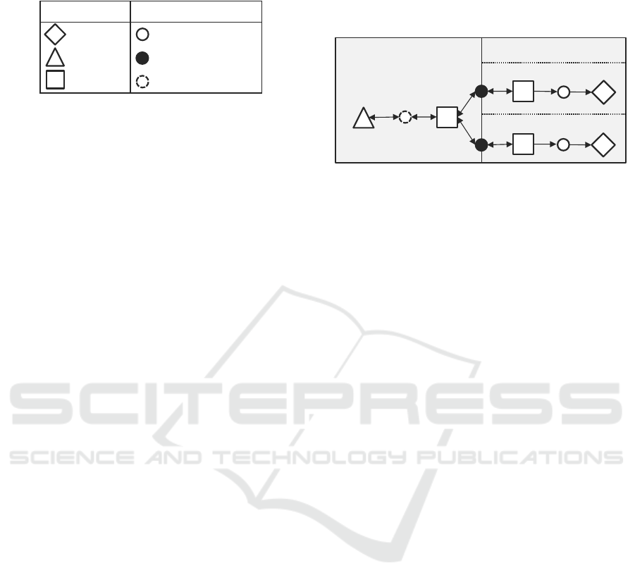
Table 2: Representation of the different symbols of

activities and states.

By mapping the logistics process with activities

and states, it is possible to build up a structure

diagram of the logistics system, which helps to

comprehensively understand the process and data

(Figure 2). Depending on the available I-points within

the material flow system, a structure diagram can be

created with varying levels of detail. This results in a

representation of a real logistics system, which serves

as a starting point for further analysis. Based on the I-

points, KPIs can be assigned to specific activities.

Thus, fundamental KPIs, including “mean

throughput”, “mean lead time”, and “mean work in

progress”, can be determined based on Little’s Law

(Little and Graves, 2008). It is noteworthy that having

two of these KPIs allows the calculation of the third.

These KPIs are important performance indicators of

logistics processes and can be calculated based on

transfer orders. The throughput (number of completed

material movements per completed period) can be

calculated for each logistics system based on transfer

orders and describes the achieved system

performance. Furthermore, availabilities may also be

determined if data is available. Consequently,

depending on the aggregation levels, these KPIs can

be identified for elements, subsystems, and the

overall system.

Based on the two key goals, the throughput is used

as the target KPI for this approach. It is crucial to

identify the influencing factors that impact the

throughput. This can be achieved by utilizing the

structure diagram and specifying cause-effect

relationships, particularly regarding the fundamental

KPIs. The next task is to quantify these influencing

factors by measurable KPIs. Various types of data and

information from different information systems and

domain knowledge can be used. As shown in Figure

2, based on the information gained from the structure

diagram, it is possible to extract data for KPI

calculation of the whole system (e.g., warehouse

system “AB”), subsystem (e.g., picking system “B”),

and element (e.g., picking stations “B1” and “B2”).

Also, forming new KPIs by conducting mathematical

operations (e.g., mean, standard deviation, etc.) with

available data or already calculated KPIs is possible

(Wuddi and Fottner, 2020). Within the literature, a

comprehensive overview of KPIs is available to offer

guidance (Dörnhöfer et al., 2016; VDI-4490, 2007).

The specific selection of KPIs depends on the

considered process and available data.

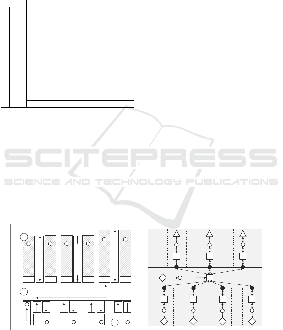
Figure 2: Structure diagram of an exemplary order picking

material flow process from storage to picking stations with

different activities and states, as well as a subdivision into

subsystems and elements.

Logistics planning and control aim to optimize

throughput by adjusting processes, parameters, and

their interactions. Therefore, continuous adjustments

to various parameters become crucial. These

variables are also essential for the evaluation of

system performance and need to be identified. These

include, for instance, working hours with shifts and

break times. Operating organization strategies (e.g.,

movement or allocation strategies, etc.) can be

approximated from data and enhanced by domain

knowledge. The actual system performance measured

by throughput also depends on the workload. This

means that if the workload is low, the system

performance will also be low. Furthermore, the

workload can be used to identify the backlog,

indicating whether and how many orders still need to

be processed. The workload and backlog can be

defined by comparing the target and actual delivery

times and thereby deducing the outstanding orders

(Lödding and Rossi, 2013). As illustrated above,

information regarding malfunctions is relevant as

well. As a result, the availabilities of subsystems and

the overall availability of the logistics system can be

determined (VDI-3581, 2004). Consequently,

external (e.g., declining customer demand) and non-

process-flow-specific factors (e.g., conveyor

breakdowns, etc.) can be considered when evaluating

the system performance.

In order to convert the low-level raw data into

KPIs, data must be cleaned (e.g., Not a Number

(NaN) values removed, etc.) and preprocessed (e.g.,

storage locations converted into distances, etc.).

Afterward, first visualizations (e.g., scatter plots, etc.)

and statistical methods (e.g., correlation analyses,

etc.) can be performed for a better understanding of

data or to identify patterns.

StateActivity

I-PointHandling

Prospected I-PointStore

Deduced StateTransfer

Data-Driven Process Analysis of Logistics Systems: Implementation Process of a Knowledge-Based Approach

For the further phases, creating a homogeneous

data set to compare individual system performances

is crucial. Thus, it is necessary to delete those entries

that generate incorrect or inaccurate KPIs. This can

be done by removing data, e.g., outside the regular

working time or during breaks and shift changes. In

future work, detailed steps will be explored.

3.2 Phase 2: Identification of

Weaknesses

Phase 2 aims to automatically detect low-performing

working periods by employing a system of

interdependent effects (Figure 3).

Figure 3: Representation of the system of interdependent

effects with key components, system variables, and

controlled variables.

The actual system performance indicates the

throughput achieved in a working period. In

comparison, the target system performance contains

the orders processed in this working period. The

theoretical system performance is approximated by

past top performance of the overall system with

similar boundary conditions (e.g., number of

conveyors, number of employees, etc.) after an outlier

elimination. The outlier elimination should be

performed as follows: Values that exceed the

threshold of 𝑞



+ 1.5 ∙ 𝑑 , where 𝑞



is the third

quartile value and 𝑑 is the interquartile range, are

removed (Krzywinski and Altman, 2014).

When determining the system variables, the order

structure must be considered. In some instances, there

is a one-to-one order structure relationship between

different subsystems, where one movement in

subsystem "A" corresponds to exactly one movement

in subsystem "B". In this case, the theoretical system

performance should be calculated for each subsystem

to get specific values. After that, the overall

theoretical system performance is determined by the

lowest maximum performance among all subsystems.

If the order structure differs, e.g., one stacker crane

run can lead to multiple picking tasks, all system

variables must be calculated separately for both

subsystems “A” and “B”.

After calculating the system variables, the

controlled variables can be evaluated. This allows to

identify unfavorable working periods. In this case, the

level of target achievement is the quotient between

actual and target system performance. It shows

whether all orders to be processed have been

processed or whether there is a backlog. The actual

level of utilization describes how close the current

system was to its past peak performance by similar

boundary conditions (e.g., capacity size), and it is

calculated by dividing actual through theoretical

systems performance. The planned level of utilization

shows the quotient of the target divided by the

theoretical system performance. It provides

information on whether the system was over- or

undersized concerning the workload. This allows an

assessment by thresholds of the three control

variables in two categories (favorable or unfavorable)

for each working period. If the control variables are

calculated for each subsystem due to the different

order structure relationships (see above). In this case,

it must be determined whether the control variables

for subsystems "A" and "B" should be unfavorable or

favorable to evaluate the working period. Due to

different logistics systems applications and

industries, the threshold values must be adapted

individually for each system. Statistical methods,

such as quantiles, can provide orientation to define

these thresholds.

The results of the control variables evaluation of

a working period are stored with all KPIs and relevant

process information (from phase 1) in a so-called

result log. They are evaluated regularly (e.g., every

week, etc.). Thus, only those working periods can be

considered where at least one or more control

variables are unfavorable. In the next step, these

working periods are automatically classified into

different problem areas using an ML model.

3.3 Phase 3: Machine Learning-Based

Identification

The objective of Phase 3 is the automated

classification of problems for further analysis. These

results can be used to evaluate and adjust correcting

actions and reduce failures to meet the key goals

mentioned. Therefore, classes must be defined before

the ML training phase starts. The classes may vary

depending on the extracted KPIs and process

information and are intended to describe specific

high-level terms of problem areas. These classes are

Approximation by

historical data

Key components

Direction of impact

System

variable

Control

variable

Reference

variable

Difference

Order

management

Targ e t Syste m

performance

Theoretical System

performance

Actual System

performance

Actual Level of

Utilization

Work load

Level of Target

achievement

Planned Level of

Utilization

Logistics

system

ICEIS 2024 - 26th International Conference on Enterprise Information Systems

used in the first step to manually evaluate the working

periods in the result log for further application of ML.

Based on the preprocessed KPIs and process

information (further called features), a process expert

can now determine reasons for unfavorable rated

working periods and assign each entry to an

appropriate class (further called labels). In this way,

meaningful relationships among KPIs can be

integrated with domain knowledge. The individual

labels can contain one or more KPIs as features and

represent unique root causes or combine several. It is

important that the classes are as heterogeneous as

possible, but the entries within a class should be

homogeneous. If entries in the results log cannot be

assigned to a unique label due to the inadequacy of

multiple KPIs, adding an additional class for these

entries should be considered. The labeled data set can

then be further processed with ML. For this purpose,

information such as date, shift name, or weekday

names must be encoded in numerical values. Since

this is a multiclass classification problem based on

labeled data, the algorithm is limited to supervised

learning classifiers.

Afterward, the ML model is trained with the

existing process information and KPIs (=features)

and the defined classes (=labels). In doing so, it is

crucial to select appropriate features (Joshi, 2020).

Due to the high complexity, the process expert can

only use some features for labeling. It is possible,

however, that using additional features will improve

the ML results. This implies that additional

relationships can be explored within the data. The

trained model should then be validated using a test

set. Frequently used metrics for validation are

Precision, Recall, F1-score, and Accuracy (Joshi,

2020). As this is a multiclass classification problem,

the ML metrics for each label can be different. If

individual labels are not predicted well, the classes

can be rechecked. For this purpose, the predicted

labels can be compared with those defined by the

process expert. Extracting the feature importance of

the trained ML model can support a better feature

selection. If no improvement is achieved, over- and

undersampling can be applied (Han et al., 2012).

Feature engineering, such as scaling, can address

varying feature scales and enhance results.

Before the actual operational mode starts, the

trained ML model must be applied to unknown data.

If the results are insufficient, the model should be

improved to provide reliable results. This can be done

by extending the data set or improving the label

assignment. Other algorithms and further data

preprocessing steps could also be applied to improve

the classification. In the operational mode, the trained

ML model automatically assigns KPIs of a working

period to a problem class. Subsequently, an overview

can be created of which and how often classes

occurred in the available data. The results show,

which problems frequently occur in the respective

analysis period. This forms the basis for further

detailed analysis in the next step.

3.4 Phase 4: Description of

Recommendations for Action

Based on the classified problem areas, a detailed

analysis of the problems is carried out in Phase 4. The

relationship between KPIs, process knowledge, and

the assignment of problem classes to specific causes

is further analyzed in this section. By the completion

of the previous phases, the raw transaction data and

transfer orders have been processed and filtered step

by step. As a result, unfavorable working periods

were identified and assigned to specific problem

classes. The procedure for root cause identification is

as follows. A label identifies one or more KPIs of a

specific problem class. Once these KPIs have been

identified, two strategies, further referred to as

strategies X and Y can be used to specify the cause.

For strategy X, it is necessary to check whether the

KPIs can be assigned to individual subsystems (e.g.,

the average distance of the entire warehouse to the

average distance of a lane). By doing so, it can be

checked if a problem affects the whole system (e.g.,

each lane of the automated storage system) or only a

part (e.g., one lane). Strategy Y corresponds to

whether the affected KPI consists of further

parameters (e.g., ratio of stock placement to stock

removal). Here, it can be identified which parameter

deviates particularly strongly. By doing so, the search

for specific causes can be narrowed down. For the

development of specific problem solutions, the

following steps can be provided. Table 3 shows the

relevant main categories of correcting actions and

disruptions, which can be divided into subcategories.

Examples are given as a guideline for the various

subcategories. Different DS methods can be applied

during the detailed analysis of specific problem areas.

Besides correlation or cluster analysis, time series

analysis can also be used to find patterns in data. This

can be used to check whether specific problems only

occur on certain working days or shifts. The steps are

characterized by a continuous exchange and a strong

input of domain knowledge from process experts.

Specified and standardized analyses can provide

support. Subsequently, measures can be taken to

increase the performance of the system or reduce

costs. The ongoing application of the approach

Data-Driven Process Analysis of Logistics Systems: Implementation Process of a Knowledge-Based Approach

presented in this article initiates a continuous

improvement process.

Table 3: Presentation of possible action recommendations

for identified problems with examples.

4 CASE STUDY

4.1 Description of the Case Study

The utilized dataset comprises transfer orders

processed by a “goods-to-person” picking system

over a span of 57 working days. Primary working

days are from Monday to Friday, with an early and a

late shift. In some cases, work is also carried out on

Saturdays. The logistics system being analyzed

comprises an automated storage and retrieval system

consisting of three lanes equipped with two racks and

one stacker crane for each lane. Additionally, there

are four picking stations in the system. There are

about 15,000 storage locations in total. The articles

are stored in standardized small load carriers that

contain up to eight sectors. Figure 4 shows the main

components of the system: (C) the different stacker

cranes and racks, (A) the different picking stations,

and (B) the material flow loop, which connects the

automated storage and retrieval system with the

picking stations. The arrows indicate the material

flow directions. A transfer order contains the

following information: Activity type (to-bin/from-

bin), storage location number, article number, article

description, loading aid number, order quantity,

order number, timestamp (time and date), and worker

identification number processed. The orders are

transferred from a warehouse management system to

the material flow computer. After a picker has called

up an order, the items to be retrieved are transported

to the respective picking station. Based on this

information, a structure diagram was built (Figure 4

right). The transfer orders allow the separation of the

overall system into subsystems (A) and (C).

Subsystem (C) describes the storage and conveyor

system, and subsystem (A) the order picking. After

the process analysis, KPIs (see Table 4) were

extracted from the data.

The preprocessing and computation of data were

conducted within a Python environment, utilizing

libraries including pandas, NumPy, and scikit-learn,

among others. Moreover, the ML models employed

were also sourced from scikit-learn.

As detailed in Section 3.1, the focus is on

identifying a comprehensive range of factors

influencing the throughput. The data was

preprocessed as follows. Individual entries with NaN-

Figure 4: Illustration of the considered logistics system (goods-to-person), including storage locations, stacker cranes, input

(il) and output location (ol), picking stations, the material flow directions, as well as I-points. The illustration a) on the left

shows the real system, whereas b) on the right the structure diagram is shown.

Picking

Stacker crane1

Stacker crane 2

Stacker crane 3

Rack 1

Rack 2

Rack 3

Rack 4

Rack 5

Rack 6

il 1 ol 2 il 1

ol 2 il 1

ol 2

i i i

iiii

i i

C2 C3

A4A3

Subcate

ories Examples

Correcting actions and disruptions

Workload

Order release Adjustment of the order

release policy

Order mix Prioritization of from-bin

orders

during high workload

… …

Operating

organization

Capacity

mana

ement

Adjustment of the number of

ees

or each shi

Allocation

strate

Verification of optimal article

zonin

… …

Disruptions

Number of

disru

tions

Identification of frequently

occurrin

disru

tions

Duration of

disruptions

Identification of disruptions

with long duration

… …

ICEIS 2024 - 26th International Conference on Enterprise Information Systems

values were removed. For each storage location

number, a distance from the storage location to the

input and output location was calculated. The x- and

y-coordinates were considered with the storage height

and width data, and the distance to the input and

output location was calculated. All entries before the

start of the early shift (before 06:00 a.m.) and after the

end of the late shift (after 11:00 p.m.) were removed.

Entries were deleted during shift changeovers

between 02:00 p.m. and 03:00 p.m. because certain

KPIs and process information (e.g., number of

employees) cannot be calculated or assigned during

this time. After this, KPIs and process information

shown in Table 4 were considered, which can be used

as features.

Table 4: Case study feature set separated into categories.

Category Features

Time-related

Datetime in hours

Date

Weekday

Shift (early and late shift)

Performance-

Number of warehouse movements per hour (h)

Number of to-bin movements per h

Number of from-bin movements per h

To-bin from-bin ratio

(Bin) occupancy-

Average distance per lane

Average distance of all lanes

Ratio of front to rear storage spaces per lane

Ratio of front to rear storage spaces of all lanes

Variation coefficient of lane utilization

Capacity-related

Number of employees per h

Number of employees to-bin movements per h

Number of employees from-bin movements per h

Mean working time per employee (to-bin)

Mean working time per employee (from-bin)

Mean time availability of all employees

Order-related

Mean lead time for a from-bin movement

Mean lead time for a picking task

Mean lead time for an all-movements task

Average inbound storage quantity

Average picking quantity

Ratio of different loading aid numbers

Subsequently, the system variables of the system

of interdependent effects described in section 3.2

were determined. Since no information regarding the

required workload was available, the level of target

achievement was always fulfilled. The actual and

planned level of utilization was used to evaluate the

system's performance. The theoretical system

performance was calculated after an outlier

elimination (see section 3.2). Since the theoretical

picking station system performance is smaller than

the theoretical conveyor system performance, this

was used as the overall theoretical system

performance. The thresholds were set to <0.8 for an

unfavorable actual and planned level of utilization for

simplification purposes. This allowed 783 out of 810

results log entries to be identified as unfavorable

working periods. In these working periods, both the

actual and planned levels of utilization were

unfavorable. Based on the process knowledge and

KPIs, five labels have been defined to classify the

data: “capacity", "storage location allocation", "order

load", "order structure", and "unknown".

4.2 Result of the Application

A Random Forest Classifier (RFC), Gradient Boost

Classifier (GBC), and Multilayer Perceptron (MLP)

were tested. A randomized grid search further

selected specific hyperparameters for all models: for

RFC and GBC, maximum feature count, maximum

depth, minimum samples leaf, and minimum samples

split were used. Grid search parameters of the MLP

model were hidden layer size, alpha values, set of

activation, and set of solvers. For the MLP, the

application of a minimum-maximum scaler showed

improvements, whereas, for the decision tree

algorithms (RFC and GBC), no improvements were

made and, therefore, not applied. Due to the

imbalanced classes, over- and undersampling were

used to improve the ML training. The 783 entries in

the data set were split into a training (80%) and test

set (20%) and evaluated by cross-validation. The ML

results on the test data are shown in Table 5.

Table 5: Results of the different ML models on the test set.

model

Resampling

techniques

recision Recall

F1-

core

Accuracy

RFC

normal

0.69 0.70 0.69 0.70

oversampled

0.68 0.69 0.68 0.69

undersampled

0.62 0.60 0.60 0.60

MLP

normal

0.67 0.69 0.68 0.69

oversampled

0.68 0.66 0.66 0.66

undersampled

0.65 0.62 0.62 0.62

GBC

normal

0.69 0.70 0.69 0.70

oversampled

0.71 0.73 0.70 0.73

undersampled

0.64 0.62 0.62 0.62

Data-Driven Process Analysis of Logistics Systems: Implementation Process of a Knowledge-Based Approach

All nine models trained were applied to unseen

data. It was found that all models could classify the

classes relatively equally. However, the best model

was an oversampled GBC. This model achieved an

average accuracy of 60%, as shown in Table 6.

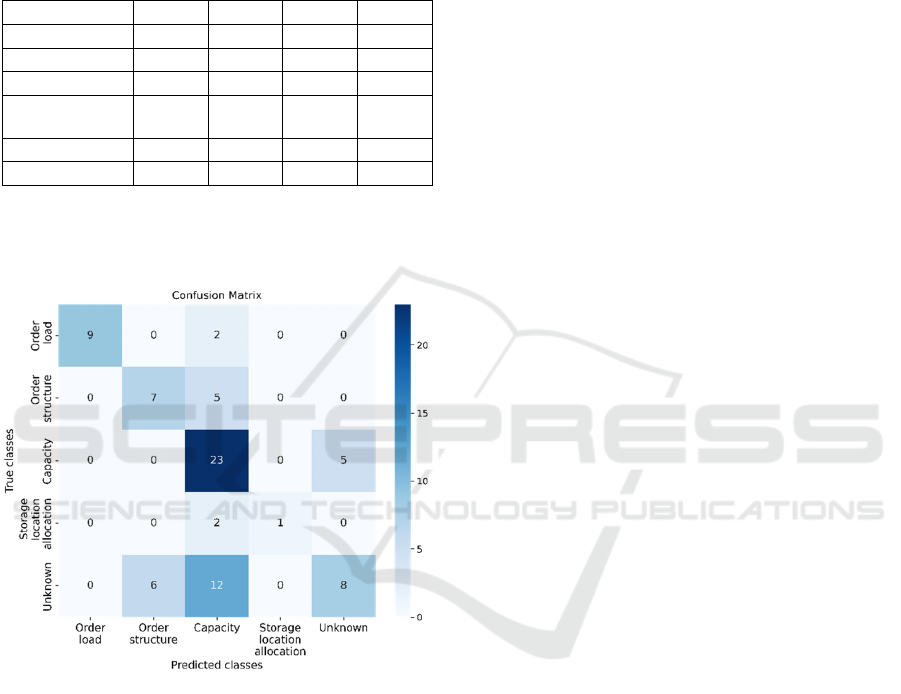
Table 6: Results of the best ML model applied to the case

study (GBC including oversampling on unseen data).

GBC Precision Recall F1-score Support

Order load

1.00 0.82 0.90 11

Order structure

0.54 0.58 0.56 12

Capacity

0.52 0.82 0.64 28

Storage location

allocation

1.00 0.33 0.50 3

Unknown

0.62 0.31 0.41 26

Accuracy

0.60 80

The following confusion matrix (Figure 5) shows

which classes are predicted well and which still have

the potential for improvement.

Figure 5: Confusion matrix for the best ML model (GBC)

on the unseen data set.

These findings suggest that the classification task

presents challenges, particularly in the case of the

"unknown" problem class. The oversimplification

may have arisen from the class definition itself.

Process experts labeled data points as "unknown"

when no specific problem could be identified for that

working period. Furthermore, "capacity" was

sometimes inaccurately classified. Numerous

misclassifications occurred due to false-negative

decisions. This phenomenon may partly be attributed

to the imbalanced data set, as this class was frequently

included in the training set. "Capacity" was the most

frequent class in the training set.

5 DISCUSSION

5.1 Interpretation

The authors suggest a design for a knowledge-based,

data-driven decision support procedure to

automatically identify performance weaknesses and

provide recommendations for improvement in

internal logistics systems using transaction data and

transfer orders. The key components of the approach

involve establishing a thorough comprehension of

processes and data, identifying relevant KPIs,

evaluating these KPIs within a system of

interdependent effects, utilizing ML to assess

unfavorable working periods, and conducting

detailed analyses of specific problems to identify root

causes. The ML classification model could classify

five different classes on unseen data with an average

accuracy of 60%. The results show that this approach

leverages low-level data, offering insights into the

analyzed process, to a more informative level that

provides a deeper understanding of problems. The

results of a case study show that ML classification

models based on process information and KPIs can

recognize the labels defined by the process expert. It

should be noted that the available data had some

shortcomings in terms of data integrity, data balance,

and data volume. Nevertheless, the application shows

that certain classes can be determined well, even with

this data. This suggests that utilizing the ongoing

application represents a method for automating

problem identification. Hence, the high degree of

automation is a significant advantage of the approach.

5.2 Limitations

Despite the confirmation of the feasibility, some

limitations have to be considered. In particular, the

approach requires a high integration of domain

knowledge to derive relevant KPIs from transaction

data to identify problems. Due to the limited data

available in the case study, important aspects such as

the equipment availability and the current workload

were not considered. This information could enhance

the robustness, precision, and content of the analysis,

enabling the identification of even more specific

problem classes. Furthermore, only problems

captured by the calculated KPIs and process

information can be identified. The use case data

shows uneven distribution. For example, there are

only three entries for the class storage location

allocation. Thus, the ML classification was validated

with a very imbalanced data set, making it difficult to

perform. However, a highly imbalanced dataset can

ICEIS 2024 - 26th International Conference on Enterprise Information Systems

also be challenging in other real-world applications.

This must be considered during the ML model

implementation using measures such as over- and

undersampling. In addition, more advanced

algorithms, such as neural networks, could improve

the results. However, it should be noted that

introducing such algorithms may increase the

complexity. Therefore, applying appropriate ML

models is crucial for a reasonable trade-off between

accuracy and complexity.

6 SUMMARY AND OUTLOOK

The authors propose a knowledge-based, data-driven

decision support procedure for process analysis in

logistics systems. The approach comprises five

phases and outlines steps to extract meaningful

insights from low-level transaction data. Validation

of the approach's usability was conducted through an

industrial case study. The identification of problems

and their root causes provides actionable

recommendations for operators of logistics systems.

Future research directions involve automating the

approach and addressing its limitations. Exploring

more detailed recommendations for action is essential

as well. Additionally, incorporating analytical

calculations as a plausibility check warrants

investigation to minimize errors in KPI determination

and enhance result accuracy.

ACKNOWLEDGEMENTS

This research was supported by KIProLog project

funded by the Bavarian State Ministry of Science and

Art (FKZ: H.2-F1116.LN33/3).

REFERENCES

Buschmann, D., Enslin, C., Elser, H., Lütticke, D., &

Schmitt, R. H. (2021). Data-driven decision support for

process quality improvements. Procedia CIRP, 99,

313–318. https://doi.org/10.1016/j.procir.2021.03.047

Chapman, P., Clinton, J., Kerber, R., Khabaza, T., Reinartz,

T. P., Shearer, C., & Wirth, R. (2022). CRISP-DM 1.0:

Step-by-step data mining guide.

Cioffi, R., Travaglioni, M., Piscitelli, G., Petrillo, A., &

Felice, F. de (2020). Artificial Intelligence and Machine

Learning Applications in Smart Production: Progress,

Trends, and Directions. Sustainability, 12(2), 492.

https://doi.org/10.3390/su12020492

Dörnhöfer, M., Schröder, F., & Günthner, W. A. (2016).

Logistics performance measurement system for the

automotive industry. Logistics Research, 9(1).

https://doi.org/10.1007/s12159-016-0138-7

Fayyad, U., Piatetsky-Shapiro, G., & Smyth, P. (1996).

From Data Mining to From Data Minin to Knowledge

Discovery in Databases. AI Magazine, 17(3).

Gröger, C., Niedermann, F., & Mitschang, B. (2012). Data

Mining-driven Manufacturing Process Optimization. In

S. I. Ao (Ed.), Lecture notes in engineering and

computer science: Vol. 3. The 2012 International

Conference of Manufacturing Engineering and

Engineering Management, the 2012 International

Conference of Mechanical Engineering (pp. 1475–

1481). Hong Kong: IAENG.

Han, J., Kamber, M., & Pei, J. (2012). Data Mining:

Concepts and Techniques. https://doi.org/10.1016/

C2009-0-61819-5

Joshi, A. V. (2020). Machine learning and artificial

intelligence. Cham.

Knoll, D., Reinhart, G., & Prüglmeier, M. (2019). Enabling

value stream mapping for internal logistics using

multidimensional process mining. Expert Systems with

Applications, 124, 130–142. https://doi.org/10.1016/

j.eswa.2019.01.026

Krzywinski, M., & Altman, N. (2014). Visualizing samples

with box plots. Nature Methods, 11(2), 119–120.

https://doi.org/10.1038/nmeth.2813

Little, J. D. C., & Graves, S. C. (2008). Little's Law. In F.

S. Hillier, D. Chhajed, & T. J. Lowe (Eds.),

International Series in Operations Research &

Management Science. Building Intuition (Vol. 115,

pp. 81–100). Boston, MA: Springer US.

https://doi.org/10.1007/978-0-387-73699-0_5

Lödding, H., & Rossi, R. (2013). Handbook of

manufacturing control: Fundamentals, description,

configuration. Berlin, Heidelberg.

Muehlbauer, K., Rissmann, L., & Meissner, S. (2022a).

Decision Support for Production Control based on

Machine Learning by Simulation-generated Data. In

Proceedings of the 14th International Joint Conference

on Knowledge Discovery, Knowledge Engineering and

Knowledge Management (pp. 54–62). SCITEPRESS -

Science and Technology Publications. https://doi.org/

10.5220/0011538000003335

Muehlbauer, K., Wuennenberg, M., Meissner, S., & Fottner,

J. (2022b). Data driven logistics-oriented value stream

mapping 4.0: A guideline for practitioners. IFAC-

PapersOnLine, 55(16), 364–369.

https://doi.org/10.1016/ j.ifacol.2022.09.051

Schuh, G., Reinhart, G., Prote, J.-P., Sauermann, F.,

Horsthofer, J., Oppolzer, F., & Knoll, D. (2019). Data

Mining Definitions and Applications for the

Management of Production Complexity. Procedia

CIRP, 81, 874–879. https://doi.org/10.1016/j.procir.20

19.03.217

Schuh, G., Reuter, C., Prote, J.-P., Brambring, F., & Ays, J.

(2017). Increasing data integrity for improving decision

making in production planning and control. CIRP

Data-Driven Process Analysis of Logistics Systems: Implementation Process of a Knowledge-Based Approach

Annals, 66(1), 425–428. https://doi.org/10.1016/

j.cirp.2017.04.003

Tao, F., Qi, Q., Liu, A., & Kusiak, A. (2018). Data-driven

smart manufacturing. Journal of Manufacturing

Systems, 48, 157–169. https://doi.org/10.1016/

j.jmsy.2018.01.006

Ungermann, F., Kuhnle, A., Stricker, N., & Lanza, G.

(2019). Data Analytics for Manufacturing Systems – A

Data-Driven Approach for Process Optimization.

Procedia CIRP, 81, 369–374. https://doi.org/

10.1016/j.procir.2019.03.064

Usuga Cadavid, J. P., Lamouri, S., Grabot, B., Pellerin, R.,

& Fortin, A. (2020). Machine learning applied in

production planning and control: a state-of-the-art in

the era of industry 4.0. Journal of Intelligent

Manufacturing, 31(6), 1531–1558. https://doi.org/

10.1007/s10845-019-01531-7

Verein Deutscher Ingenieure (September 2015).

Warehouse-Management-Systeme. (VDI-Richtlinie,

VDI-3601). Berlin: Beuth Verlag GmbH.

Verein Deutscher Ingenieure e.V. (2004). Availability of

transport and storage systems including subsystems

and elements. (Richtlinie, VDI-3581). Berlin: Beuth

Verlag GmbH.

Verein Deutscher Ingenieure e.V. (2007). Operational

logistics key figures from goods receiving to dispatch.

(Richtlinie, VDI-4490). Berlin: Beuth Verlag GmbH.

Wuddi, P. M., & Fottner, J. (2020). Key Figure Systems. In

Proceedings of the 2020 International Conference on

Big Data in Management (pp. 125–129). New York,

NY, USA: ACM. https://doi.org/10.1145/343707

5.3437090

Wuennenberg, M., Muehlbauer, K., Fottner, J., & Meissner,

S. (2023). Towards predictive analytics in internal

logistics – An approach for the data-driven

determination of key performance indicators. CIRP

Journal of Manufacturing Science and Technology, 44,

116–125. https://doi.org/10.1016/j.cirpj.2023.05.005

ICEIS 2024 - 26th International Conference on Enterprise Information Systems