Generalizing Conditional Naive Bayes Model
Sahar Salmanzade Yazdi
1
, Fatma Najar
2
and Nizar Bouguila
1
1
Concordia Institute for Information Systems Engineering (CIISE),
Concordia University, Montreal, QC., Canada
2
City University of New York (CUNY), John Jay College, New York, NY, U.S.A.
Keywords:
Conditional Naive Bayes Model (CNB), Latent Dirichlet Allocation (LDA), LD-CNB Model, LGD-CNB
Model, LBL-CNB Model.
Abstract:
Given the fact that the prevalence of big data continues to evolve, the importance of information retrieval tech-
niques becomes increasingly crucial. Numerous models have been developed to uncover the latent structure
within data, aiming to extract necessary information or categorize related patterns. However, data is not uni-
formly distributed, and a substantial portion often contains empty or missing values, leading to the challenge
of ”data sparsity”. Traditional probabilistic models, while effective in revealing latent structures, lack mech-
anisms to address data sparsity. To overcome this challenge, we explored generalized forms of the Dirichlet
distributions as priors to hierarchical Bayesian models namely the generalized Dirichlet distribution (LGD-
CNB model) and the Beta-Liouville distribution (LBL-CNB model). Our study evaluates the performance
of these models in two sets of experiments, employing Gaussian and Discrete distributions as examples of
exponential family distributions. Results demonstrate that using GD distribution and BL distribution as priors
enhances the model learning process and surpass the performance of the LD-CNB model in each case.
1 INTRODUCTION
In the realm of unsupervised learning, the structure
of the data remains hidden from the observer which
prompted the development of probabilistic mixture
models. Indeed, a powerful approach aimed at fig-
uring out this hidden structure, given that the data
comprises a mixture of multiple underlying compo-
nents (Li et al., 2016). Naive-Bayes (NB) models are
a type of generative mixture models known for their
simplicity, accuracy, and speed, making them widely
used in tasks like product recommendations, medical
diagnoses, software defect predictions, and cyberse-
curity. In addition, researchers have shown that these
models tend to outperform other approaches, such
as C4.5, PEBLS, and CN2 classifiers especially in
cases with small datasets (Wickramasinghe and Ka-
lutarage, 2021). In the era of big data, it is com-
mon to encounter issues like sparsity, missing val-
ues, and unobserved data. This is often due to the
fact that users have limited knowledge about the vast
number of available items. Hence, employing tradi-
tional NB models won’t be advantageous when deal-
ing with such large-scale datasets. To tackle the spar-
sity problem, a generalized form of the Naive Bayes
model, referred to as the conditional Naive Bayes
(CNB) model, was introduced (Taheri et al., 2010).
This model calculates the likelihood of each class for
a given feature vector by utilizing a subset of observed
features, rather than incorporating all of them, thus
addressing the sparsity problem. However, unlike
the traditional Naive Bayes model, the CNB model
does not consider the assumption of feature indepen-
dence. To tackle this limitation, alternative mod-
els were suggested including multi-case model (Sa-
hami et al., 1996), overlapping mixture model (Fu
and Banerjee, 2008), aspect model (Hofmann, 2001),
LDA (Blei et al., 2003), and LD-CNB model (Baner-
jee and Shan, 2007). Latent Dirichlet Allocation
(LDA) is a probabilistic generative model of a corpus,
where documents are represented as random mixtures
over latent low-dimensional topic space. Assuming
K latent topics, a document is generated by sam-
pling a mixture of these topics, with each topic rep-
resented as a probability distribution over the words
in the document, and then sampling words from that
mixture. The key aspect of LDA is that despite the
CNB model, it allows documents to be associated
with two or more topics (Blei et al., 2003). The latent
Dirichlet conditional Naive-Bayes (LD-CNB) model
was presented as a more adaptable model since it
Yazdi, S., Najar, F. and Bouguila, N.
Generalizing Conditional Naive Bayes Model.
DOI: 10.5220/0012524000003690
Paper published under CC license (CC BY-NC-ND 4.0)
In Proceedings of the 26th International Conference on Enterprise Information Systems (ICEIS 2024) - Volume 1, pages 163-171
ISBN: 978-989-758-692-7; ISSN: 2184-4992
Proceedings Copyright © 2024 by SCITEPRESS – Science and Technology Publications, Lda.
163

utilizes exponential family distribution in variational
approximation for model inference and learning. In
the research conducted by Banerjee et al.(Banerjee
and Shan, 2007), they applied Gaussian and Discrete
distributions as specific examples of such exponen-
tial family distributions. Through a comparison be-
tween the LD-CNB and the CNB models, it has been
demonstrated that the LD-CNB model consistently
outperforms the CNB model in terms of having lower
perplexity. However, using Dirichlet as a prior distri-
bution in the model can lead to some constraints. To
address the limitations associated with the constrict-
ing negative covariance structure of Dirichlet distribu-
tion, this paper introduces an approach where we sug-
gest employing alternative distributions, specifically
the generalized Dirichlet (GD) distribution and the
Beta-Liouville (BL) distribution, as priors to define
the mixing weights for the data point in the model.
The paper’s organization is as follows: In section
2, we provide an overview of the LD-CNB model,
its instantiations for exponential family distributions
such as Gaussian and Discrete distributions, and the
variational Expectation Maximization algorithm used
for learning and inference. Section 3 covers a re-
view of the properties of the generalized Dirichlet
(GD) distribution and the Beta-Liouville (BL) dis-
tribution, our proposed approaches, and the updated
model based on each of those prior distributions. Sec-
tion 4 presents the experimental results obtained from
the UCI benchmark repository (Frank, 2010) and
Movielens recommendation system dataset (Harper
and Konstan, 2015). Finally, in section 5, we offer
our conclusions.
2 LATENT DIRICHLET
CONDITIONAL NAIVE BAYES
In this section, we will examine the LD-CNB model
and discuss the constraints of both the LDA model
and the Naive-Bayes model, which led to the devel-
opment of LD-CNB. Additionally, we will delve into
the details of the variational EM algorithm and the
computational steps taken to accomplish the goals of
model learning and inference.
The LD-CNB model was proposed in response
to the limitations of NB models in handling sparsity
within large-scale data sets. Because the observer
has limited knowledge regarding the magnitude of the
items, the likelihood of encountering missing or un-
observed values rises. Although NB models demon-
strated their accuracy and ability in processing small
datasets, they are still not able to handle the sparsity
in the case of big data. Furthermore, in the NB model,
it is assumed that features come from a single mixture
component, which imposes significant limitations on
the modeling capabilities of the NB model.
In order to address the challenges associated with
sparsity, the Conditional Naive-Bayes (CNB) model
was introduced. This model conditions a Naive-Bayes
model on only a subset of observed features. Let’s
assume that d represents the total number of fea-
tures in the dataset, a subset of features is denoted
as f = { f
1
,..., f
m
}, where m < d. The conditional
probability of the feature vector x is then computed as
follows:
p(x|π,Θ, f ) =
K
∑
z=1
p(z|π)
m
∏
j=1
p
ψ
(x
j
|z,Θ, f
j
)
(1)
where π represents prior distribution over K compo-
nents. The term ψ refers to the appropriate exponen-
tial family model for feature f
j
and p
ψ
(x
j
|z,Θ, f
j
)
is the exponential family distribution for f
j
. z =
(1,...,K) and Θ = {θ
z
} are defined as the parameters
for the exponential family distribution.
In the context of LDA, a ’data point’ is presented
as a sequence of tokens (feature), with each token
generated from the same discrete distribution, since
they are considered semantically identical (Griffiths
and Steyvers, 2004). In some applications, instead of
considering a feature as a token, each feature is as-
sociated with a measured value, which can be real or
categorical. Besides that, various features within the
feature set can carry distinct semantic meanings. Be-
cause the NB model assumes that features come from
the same mixture component, they took a Dirichlet
prior with parameter α for the mixing weight π to
overcome the problem caused by that assumption.
Therefore, the process of generating a sample x fol-
lowing the LD-CNB model can be outlined as fol-
lows:
1. Choose π ∼ Dir(α)
2. For each of the observed feature f
j
( j=1, ..., m):
(a) Choose z
j
∼ Discrete(π)
(b) Choose a feature value x
j
∼ p
ψ
(x
j
|z
j
,Θ, f
j
)
When taking the model parameters into account,
the joint distribution of (π, z, x) can be expressed as:
p(π,z,x|α,Θ, f ) = p(π|α)
m
∏
j=1
p(z
j
|π)p
ψ
(x
j
|z
j
,Θ, f
j
)
(2)
Given the feature set of the entire data set denoted
as F = { f
1
,..., f
N
}, the probability of the entire data
set X = {x
1
,...,x
N
} can be calculated as follows:
ICEIS 2024 - 26th International Conference on Enterprise Information Systems
164

p(X|α, Θ, f ) =
N
∏
i=1
Z
π
p(π|α)
m
i
∏
j=1
K
∑
z
i j
=1
p(z
i j
|π)p
ψ
(x
i j
|z
i j
,Θ, f
i j
)
!
dπ
(3)
It can be seen from Equation 3, that the model is
dependent on the observed features and their poten-
tial values. Thus, when generating the value x
j
for the
feature f
j
, it is necessary to select the suitable expo-
nential family model (ψ). It’s important to note that
the choice of family distribution depends on the spe-
cific feature because each feature may have a different
family distribution.
In the research conducted by Banerjee et
al.(Banerjee and Shan, 2007), they utilized a uni-
variate Gaussian distribution for real-valued fea-
tures and a Discrete distribution for categorical fea-
tures within each class. For the Gaussian distribu-
tion model (LD-CNB-Gaussian), the model param-
eters are denoted as Θ = {(µ
(z, f
j
)
,σ
2
(z, f
j
)
)}, where
j = 1,...,d, and z = 1,...,K (d and K representing
the total number of features and the number of la-
tent classes in the dataset, respectively). Therefore,
in equation 3, p
ψ
(x
i j
|z
i j
,Θ, f
i j
) can be updated as
p(x
j
|µ
(z, f
j
)
,σ
2
(z, f
j
)
). In the case of Discrete distribu-
tion (LD-CNB-Discrete model), each feature is al-
lowed to be of a different type and a different num-
ber of possible values. Assuming K latent classes
(z = 1, ...,K), and d features with r
j
( j = 1,...,d) pos-
sible values for each feature, the model parameters
for latent class z and feature f
j
are represented by
discrete probability distribution over possible values
Θ = {p
(z, f
j
)
(r)}, where r = (1,...,r
j
).
2.1 Model Learning and Inference
2.1.1 Variational EM Algorithm
Consider y as the observed data generated through a
set of latent variables x. Let Θ denotes the model
parameter describing the dependencies between vari-
ables. Consequently, the likelihood of observing the
data can be expressed as a function of Θ. The objec-
tive is to identify the optimal value for Θ that maxi-
mizes the likelihood, or equivalently, the logarithm of
the likelihood, as illustrated in equation 4.
log p(y|Θ) = log
Z
p(x,y|Θ)dx (4)
However, the computation of maximum log-
likelihood is typically a complex task. As a solution,
an arbitrary distribution for hidden variables, denoted
as q(x), is defined. The marginal likelihood can then
be broken down with respect to q(x) as outlined be-
low:
log p(y|Θ) = log
Z
q(x)
p(x,y|Θ)
q(x)
dx
− log
Z
q(x)
p(x|y,Θ)
q(x)
dx
= L(q(x)|Θ) + K L(q(x)||p(x|y,Θ))
(5)
The term L(q(x)|Θ) is referred to as the ev-
idence lower bound (ELBO), serving as a lower
bound for log p(y|Θ) due to the non-negativity of
K L(q(x)||p(x|y,Θ)) (Li and Ma, 2023). To achieve
the maximum log-likelihood, we can either minimize
K L(q(x)||p(x|y,Θ)) or maximize the evidence lower
bound (ELBO), denoted as L(q(x)|Θ). Consequently,
rather than directly maximizing the log-likelihood,
the focus is on maximizing the ELBO (Li and Ma,
2023). This approach leads to the development of a
variational EM algorithm, which iteratively optimizes
the lower bound of the log-likelihood.
q(π,z|γ,φ, f ) = q(π|γ)
m
∏
j=1
q(z
j
|φ
j
)
(6)
q(π,z|γ,φ, f ) is introduced as a variational distribu-
tion over the latent variables conditioned on free pa-
rameters γ and φ, where γ is a Dirichlet parameter, and
φ = (φ
1
,...,φ
m
) is a vector of multinomial parameters.
Based on the information above, the associated
ELBO can be computed as follows:
L(γ,φ; α,Θ) = E
q
[log p(π|α)] + E
q
[log p(z|π)]
+ E
q
[log p(x|z,Θ)] + H (q(π))
+ H (q(z))
(7)
The variational EM-step is derived by setting the
partial derivatives, with respect to each variational
and model parameter, to zero. The ELBO can be op-
timized iteratively by employing the following set of
update equations:
φ
(z
j
, f
j
)
∝ exp


Ψ(γ
z
j
) − Ψ(
K
∑
z
j
′
=1
γ
z
j
′
)


p
ψ
(x
j
|z
j
,Θ, f
j
)
(8)
γ
z
j
= α
z
j
+
m
∑
j=1
φ
(z
j
, f
j
)
(9)
As previously shown, the respective distributions
for LD-CNB-Gaussian and LD-CNB-Discrete will be
substituted with p
ψ
(x
j
|z
j
,Θ, f
j
) in (8). The updated
corresponding parameter (Θ) for each model is then
calculated as follows:
Generalizing Conditional Naive Bayes Model
165

• LD-CNB-Gaussain
µ
(z
j
, f
j
)
=
∑
N
i=1
φ
i(z
j
, f
j
)
x
i j
∑
N
i=1
φ
i(z
j
, f
j
)
(10)
σ
2
(z
j
, f
j
)
=
∑
N
i=1
φ
i(z
j
, f
j
)
(x
i j
− µ
(z
j
, f
j
)
)
2
∑
N
i=1
φ
i(z
j
, f
j
)
(11)
• LD-CNB-Discrete
p
(z
j
, f
j
)
(r) ∝
N
∑
i=1
φ
i(z
j
, f
j
)
x
i j
1(r|i, f
j
) + ε (12)
In equation 12, the term 1(r|i, f
j
) refers to the in-
dicator matrix of observed value r for feature f
j
in
observation x
i
.
However, using Dirichlet as a prior presents some
restrictions, especially when modeling correlated top-
ics. First, all data features are bound to share a com-
mon variance, and their sum must be equal to one.
Consequently, we cannot introduce individual vari-
ance information for each component of the random
vector. In addition, when using a Dirichlet distribu-
tion, we have only one degree of freedom to convey
our confidence in the prior knowledge. All the en-
tries in the Dirichlet prior are always negatively cor-
related which means if the probability of one compo-
nent increases, the probabilities of the other compo-
nents must either decrease or remain the same to en-
sure they still sum up to one (Caballero et al., 2012).
These limitations motivated us to employ a general-
ized form of Dirichlet distribution, namely general-
ized Dirichlet distribution, and Beta-Liouville distri-
bution as potential priors for the multinomial distribu-
tion.
3 PROPOSED APPROACHES
In this section, we provide a concise overview of
the generalized Dirichlet distribution and the Beta-
Liouville distribution. We then proceed to adjust the
equations in accordance with these new priors.
3.1 Latent Generalized Dirichlet
Conditional Naive Bayes
To overcome the limitations associated with the
Dirichlet distribution, (Bouguila and ElGuebaly,
2008; Bouguila and Ghimire, 2010), Connor and
Mosimann introduced the concept of neutrality and
developed the generalized Dirichlet distribution (Con-
nor and Mosimann, 1969) which is conjugate to the
multinomial distribution Najar and Bouguila (2022a).
In this context, a random vector
−→
X is considered com-
pletely neutral when, for all values of j ( j < K),
the vector (x
1
,x
2
,...,x
j
) is independent of the vec-
tor (x
j+1
,x
j+2
,...,x
K
)/(1 −
∑
j
(x
1
,x
2
,...,x
j
)), which
means that a neutral vector does not impact the pro-
portional division of the remaining interval among the
rest of the variables. By assuming a univariate beta
distribution with parameters α and β for each compo-
nent of (x
1
,x
2
,...,x
K−1
), the probability density func-
tion for the generalized Dirichlet distribution is de-
rived as follows:
GD(
−→
X |α
1
,...,α
K
,β
1
,...,β
K
) =
K
∏
i=1
Γ(α
i
+ β
i
)
Γ(α
i
)Γ(β
i
)
x
(α
i
−1)
i
(1 −
i
∑
j=1
x
j
)
γ
i
(13)
where
for i = 1,2,...,K − 1, γ
i
= β
i
− (α
i+1
+ β
i+1
)
and γ
K
= β
K
− 1
Note that α
i
,β
i
> 0. For i = 1,2,...,K, x
i
≥ 0 and
∑
K
i=1
x
i
≤ 1 (Epaillard and Bouguila, 2019). Assum-
ing β
i−1
= α
i
+ β
i
the generalized Dirichlet distribu-
tion is reduced to the Dirichlet distribution, which in-
dicates Dirichlet distribution as a special case of the
generalized Dirichlet distribution (Bouguila, 2008).
The mean, the variance, and the covariance in the
case of the generalized Dirichlet distribution, for i =
1,...,K − 1 are as follows:
E(X
i
) =
α
i
α
i
+ β
i
i−1
∏
j=1
β
j
+ 1
α
j
+ β
j
(14)
Var(X
i
) = E(X
i
)×
α
i
+ 1
α
i
+ β
i
+ 1
i−1
∏
j=1
β
j
+ 1
α
j
+ β
j
+ 1
− E(X
i
)
!
(15)
COV (X
i
,X
d
) = E(X
d
)×
α
i
α
i
+ β
i
+ 1
i−1
∏
j=1
β
j
+ 1
α
j
+ β
j
+ 1
− E(X
i
)
!
(16)
Unlike Dirichlet distribution, the GD distribution
has a more general covariance structure, and variables
with the same means are not obligated to have the
same covariance. Moreover, for GD distribution co-
variance between two variables is not negative (Najar
and Bouguila, 2021). This flexibility and properties
of the GD distribution make it desirable prior to the
topic modeling and finding the hidden structure of the
data (Koochemeshkian et al., 2020).
ICEIS 2024 - 26th International Conference on Enterprise Information Systems
166

3.2 Model Learning and Inference
Variational EM Algorithm. In the proposed ap-
proach, we consider a GD prior with parameters α, β
for the mixing weights of the data points of the
model (π ∼ GD(α,β)), and Θ as the model param-
eter. Therefore, the joint distribution of (π,z,x) is cal-
culated as:
p(π,z,x|α,β,Θ, f ) =
p(π|α,β)
m
∏
j=1
p(z
j
|π)p
ψ
(x
j
|z
j
,Θ, f
j
)
(17)
Following that, the variational distribution for up-
dated model parameters is defined as:
q(π,z|γ,λ,φ, f ) = q(π|γ, λ)
m
∏
j=1
q(z
j
|φ
j
)
(18)
where γ and λ are the parameters for the generalized
Dirichlet distribution, and φ = (φ
1
,...,φ
m
) denotes a
vector of parameters for the multinomial distribution.
Further, in order to determine the maximum likeli-
hood of the data, we seek to maximize the associated
lower bound (ELBO), computed as follows:
L(γ,λ,φ; α,β,Θ) =E
q
[log p(π|α,β)] + E
q
[log p(z|π)]
+ E
q
[log p(x|z,Θ)] + H (q(π))
+ H (q(z))
(19)
It has been demonstrated that the GD distribu-
tion belongs to the exponential family, so its expected
value is calculated by taking the derivative of its cu-
mulant function (Appendix A). By setting the partial
derivatives to zero with regard to each parameter and
subsequently deriving the revised equations for vari-
ational and model parameters (equations 20-22), we
can find the maximum value for the ELBO.
φ
(z
j
, f
j
)
∝ p
ψ
(x
j
|z
j
,Θ, f
j
)×
exp Ψ(γ
z
j
) − Ψ(λ
z
j
) − (
z
j
∑
i=1
Ψ(γ
i
+ λ
i
) − Ψ(λ
i
))
!
(20)
γ
z
j
= α
z
j
+
m
∑
j=1
φ
(z
j
, f
j
)
(21)
λ
z
j
= β
z
j
+
m
∑
j=1
φ
(z
j
, f
j
)
(22)
Given that the model parameter Θ form is inde-
pendent of the prior distribution, the update equations
for exponential family parameters remain unchanged,
as presented in (10-12).
3.3 Latent Beta-Liouville Conditional
Naive Bayes
In this study, we will incorporate another distribution
known as the Beta-Liouville (BL) distribution as a
prior in our model. Research has demonstrated that
the BL distribution offers a viable alternative to the
Dirichlet and GD distributions for statistically repre-
senting proportional data. The BL distribution also
serves as a conjugate prior for the multinomial dis-
tribution and, similar to the GD distribution, it has a
more general covariance structure (Luo et al., 2023).
The probability density function for a random vector
−→
X following a BL distribution with positive parame-
ter vector
−→
Φ = (α
1
,...,α
K
,α,β) is expressed as:
BL(
−→
X |
−→
Φ) =
Γ(
K
∑
k=1
α
k
)
Γ(α + β)
Γ(α)Γ(β)
K
∏
k=1
X
(α
k
−1)
k
Γ(α
k
)
×
K
∑
k=1
X
k
!
α−
∑
K
k=1
α
k
1 −
K
∑
k=1
X
k
!
β−1
(23)
The Beta-Liouville distribution transforms into
the Dirichlet distribution when the generator density
follows a beta distribution with parameters
∑
K−1
i=1
α
i
and α
K
, as explained in (Fan and Bouguila, 2015;
Bouguila, 2010). The mean, the variance, and the co-
variance of the Beta-Liouville distribution are calcu-
lated as follows:
E(X
i
) =
α
α + β
α
k
∑
K
k=1
α
k
(24)
Var(X
i
) = E(X
i
)

α + 1
α + β + 1
α
k
+ 1
∑
K
k=1
α
k
+ 1

− E(X
i
)
2

α
2
k
(
∑
K
k=1
α
k
)
2

(25)
COV (X
i
,X
d
) =
α
i
α
d
∑
K
i=1
α
i

−
α
2
(α + β)
2
∑
K
k=1
α
k
+
α(α + 1)
(α + β)(α + β + 1)(
∑
K
k=1
α
k
+ 1)

(26)
By considering a Beta-Liouville (BL) prior with
parameter vector
−→
Φ from which the mixing weight
π is generated, we compute the joint distribution of
(π,z,x), the associated variational distribution, and
the lower bound, respectively, as outlined below:
Generalizing Conditional Naive Bayes Model
167

p(π,z,x|
−→
Φ,Θ, f ) = p(π|
−→
Φ)
m
∏
j=1
p(z
j
|π)p
ψ
(x
j
|z
j
,Θ, f
j
)
(27)
q(π,z|
−→
Φ,φ, f ) = q(π|
−→
Ω)
m
∏
j=1
q(z
j
|φ
j
)
(28)
L(
−→
Ω,φ;
−→
Φ,Θ) = E
q
[log p(π|
−→
Φ)] + E
q
[log p(z|π)]
+ E
q
[log p(x|z,Θ)] + H (q(π))
+ H (q(z))
(29)
where,
−→
Ω = (γ
1
,...,γ
K
,γ,λ) is the Beta-Liouville pa-
rameter vector and φ = (φ
1
,...,φ
m
) are the multino-
mial parameters. The BL distribution is also a mem-
ber of the exponential family (Appendix B), thus
the expected value will be obtained by computing
the derivative of its cumulant function (Bakhtiari and
Bouguila, 2016). Consequently, the corresponding
variational parameters are updated as follows:
φ
(z
j
, f
j
)
∝ p
ψ
(x
j
|z
j
,Θ, f
j
)×
exp Ψ(γ
z
j
) − Ψ(
K
∑
z
j
=1
γ
z
j
) + Ψ(λ) − Ψ(γ + λ)
!
(30)
γ
z
j
= α
z
j
+
m
∑
j=1
φ
(z
j
, f
j
)
(31)
4 EXPERIMENTAL RESULTS
To evaluate the performance of our LGD-CNB and
LBL-CNB models and to compare them with LD-
CNB model for each experiment, we selected differ-
ent sets of data. This assessment examines how three
different priors affect the Gaussian and Discrete mod-
els.
4.1 Gaussian Models
As mentioned earlier, Gaussian models are suit-
able for features with real values. Table 1 displays
the calculated perplexities for LD-CNB-Gaussian,
LGD-CNB-Gaussian, and LBL-CNB-Gaussian mod-
els across five different datasets. These datasets are
chosen from the UCI benchmark repository, in which
all features are available for every instance. The
model was trained using 70% of the data, and the re-
maining 30% was utilized for testing. Perplexity val-
ues are then computed on the testing set using equa-
tion 32, with the same number of selected features for
all instances in the dataset. The perplexity values after
10 iterations are presented in Table 1. According to
equation 32, lower perplexity indicates a higher log-
likelihood probability, suggesting a better fit for the
model.
Perplexity(X) = exp
n
−
∑
N
i=1
log p(x
i
)
∑
N
i=1
m
i
o
(32)
Table 1: Perplexity of LD-CNB, LGD-CNB, and LBL-CNB
Gaussian models.
LD LGD LBL
Wine 0.9936 0.9804 0.93262
Balance 0.9966 0.9810 0.9953
HeartFailure 0.9837 0.8792 0.7987
WDBC 0.9967 0.9943 0.9925
Yeast 0.9974 0.9963 0.9959
Results indicate that LGD-CNB-Gaussian and
LBL-CNB-Gaussian models perform better than LD-
CNB-Gaussian, showing that the generalized struc-
ture of GD distribution and BL distribution makes
them more suitable as prior distributions. Table 2 dis-
plays the outcomes of assessing the models on the
WDBC dataset (Wolberg and Street, 1995). These
results represent the averages obtained from 20 runs
with distinct randomly assigned initial values. Ac-
cording to the table, both the LGD-CNB model and
LBL-CNB model outperform the LD-CNB model,
showcasing higher accuracy in those instances.
Table 2: Accuracy, precision, recall, and f-score in per-
cent for LD-CNB, LGD-CNB, LBL-CNB using the WDBC
dataset.
Accuracy Precision Recall F-score
LD 0.63 0.55 0.075 0.132
LGD 0.85 0.75 0.90 0.828
LBL 0.82 0.92 0.55 0.688
4.2 Discrete Models
To assess Discrete models, we utilized the 100K
MovieLens dataset from the Grouplens Research
Project (Harper and Konstan, 2015). This dataset
comprises 100,000 ratings (1-5) provided by 943
users for 1682 movies. Users with fewer than 20 rat-
ings or incomplete demographic information were ex-
cluded. Due to users not rating all movies, there is
sparsity in this dataset. Similar to the prior experi-
ICEIS 2024 - 26th International Conference on Enterprise Information Systems
168

ment, we conducted the experiment on our three mod-
els and computed the perplexity for each using Equa-
tion 33.
Perplexity(X) = exp
n
−
∑
N
i=1
log p(x
i
)
N
o
(33)
The disparity in the number of rated movies
among users serves as evidence for the dataset’s spar-
sity, a notable distinction between the Discrete model
and the Gaussian model. Moreover, there are no con-
straints on the covariance of data points, implying that
a user rating fewer movies does not necessitate an-
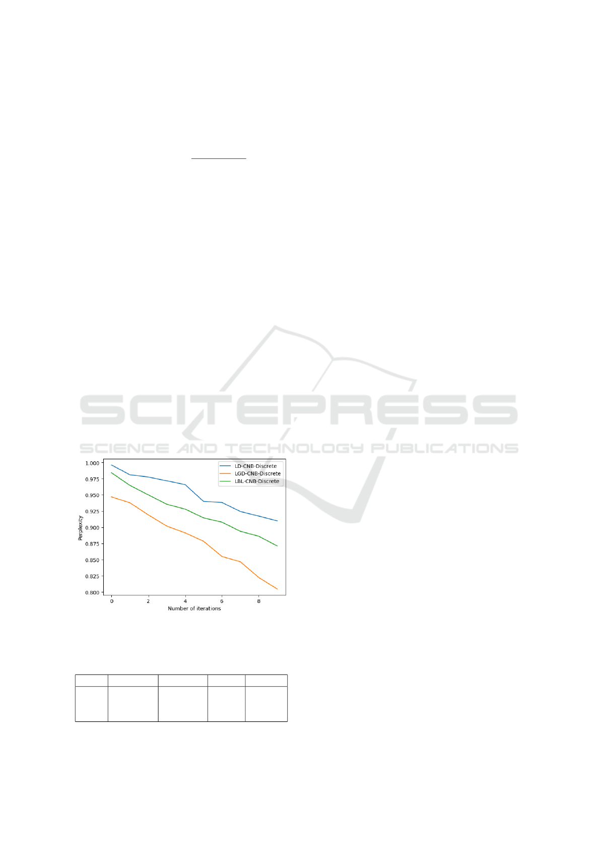
other user to rate more. As illustrated in Figure 1,
despite the sparsity, the perplexity of the LGD-CNB-
Discrete model is lower than that of the LBL-Discrete
model, which, in turn, is lower than the LD-CNB-
Discrete model. This finding suggests that similar
to real-valued features, the more general covariance
structure of the GD and BL priors allows them to bet-
ter describe proportional data, leading to their supe-
rior performance over the Dirichlet prior to categori-
cal features. Additionally, the presence of two vector
parameters in the GD distribution enhances its flexi-
bility with sparse data, enabling it to assign low val-
ues effectively (Najar and Bouguila, 2022b). In this
experiment, we compute similarly the accuracy, pre-
cision, recall, and F-score for this model using the
testing set. Table 3 illustrates that the suggested ap-
proaches have led to an enhancement in the overall
performance.
Figure 1: Perplexity for LD-CNB-Discrete, LGD-CNB-
Discrete, and LBL-CNB-Discrete.
Table 3: Accuracy, precision, recall and f-score in percent
for LD-CNB, LGD-CNB, LBL-CNB Discrete models.
Accuracy Precision Recall F-score
LD 0.83 0.62 0.052 0.095
LGD 0.87 0.75 0.51 0.607
LBL 0.86 0.74 0.39 0.51
5 CONCLUSION
In this paper, we have presented the incorporation of
the GD and BL distributions as priors in the CNB
model to address sparsity in large-scale datasets. Uti-
lizing the Conditional Naive Bayes (CNB) model, we
conditioned the model on observed feature subsets,
enhancing sparsity management. The traditional ap-
proach assumed a Dirichlet distribution as a prior,
LD-CNB acknowledges that feature values are gen-
erated from an exponential family distribution, vary-
ing depending on the considered feature. We have
outlined the advantages of employing GD and BL
distributions over the Dirichlet distribution. Our in-
vestigation into the Gaussian and Discrete distribu-
tions as exponential families for LGD-CNB and LBL-
CNB models revealed that the more generalized co-
variance structure of GD and BL distributions makes
them desirable as prior distributions for uncovering
latent structures in sparse data, especially when fea-
ture vectors follow a discrete distribution.
REFERENCES
Bakhtiari, A. S. and Bouguila, N. (2016). A latent beta-
liouville allocation model. Expert Systems with Appli-
cations, 45:260–272.
Banerjee, A. and Shan, H. (2007). Latent dirichlet con-
ditional naive-bayes models. In Seventh IEEE Inter-
national Conference on Data Mining (ICDM 2007),
pages 421–426. IEEE.
Blei, D. M., Ng, A. Y., and Jordan, M. I. (2003). Latent
dirichlet allocation. Journal of machine Learning re-
search, 3(Jan):993–1022.
Bouguila, N. (2008). Clustering of count data using gen-
eralized dirichlet multinomial distributions. IEEE
Transactions on Knowledge and Data Engineering,
20(4):462–474.
Bouguila, N. (2010). Count data modeling and classifica-
tion using finite mixtures of distributions. IEEE Trans-
actions on Neural Networks, 22(2):186–198.
Bouguila, N. (2011). Hybrid generative/discriminative ap-
proaches for proportional data modeling and classifi-
cation. IEEE Transactions on Knowledge and Data
Engineering, 24(12):2184–2202.
Bouguila, N. and ElGuebaly, W. (2008). On discrete data
clustering. In Pacific-Asia Conference on Knowl-
edge Discovery and Data Mining, pages 503–510.
Springer.
Bouguila, N. and Ghimire, M. N. (2010). Discrete visual
features modeling via leave-one-out likelihood esti-
mation and applications. Journal of Visual Commu-
nication and Image Representation, 21(7):613–626.
Caballero, K. L., Barajas, J., and Akella, R. (2012). The
generalized dirichlet distribution in enhanced topic
Generalizing Conditional Naive Bayes Model
169

detection. In Proceedings of the 21st ACM interna-
tional conference on Information and knowledge man-
agement, pages 773–782.
Connor, R. J. and Mosimann, J. E. (1969). Concepts of
independence for proportions with a generalization of
the dirichlet distribution. Journal of the American Sta-
tistical Association, 64(325):194–206.
Epaillard, E. and Bouguila, N. (2019). Data-free metrics
for dirichlet and generalized dirichlet mixture-based
hmms–a practical study. Pattern Recognition, 85:207–
219.
Fan, W. and Bouguila, N. (2015). Expectation propaga-
tion learning of a dirichlet process mixture of beta-
liouville distributions for proportional data cluster-
ing. Engineering Applications of Artificial Intelli-
gence, 43:1–14.
Frank, A. (2010). Uci machine learning repository.
http://archive. ics. uci. edu/ml.
Fu, Q. and Banerjee, A. (2008). Multiplicative mix-
ture models for overlapping clustering. In 2008
Eighth IEEE International Conference on Data Min-
ing, pages 791–796. IEEE.
Griffiths, T. L. and Steyvers, M. (2004). Finding scientific
topics. Proceedings of the National academy of Sci-
ences, 101(suppl 1):5228–5235.
Harper, F. M. and Konstan, J. A. (2015). The movielens
datasets: History and context. Acm transactions on
interactive intelligent systems (tiis), 5(4):1–19.
Hofmann, T. (2001). Unsupervised learning by probabilistic
latent semantic analysis. Machine learning, 42:177–
196.
Koochemeshkian, P., Zamzami, N., and Bouguila, N.
(2020). Flexible distribution-based regression mod-
els for count data: Application to medical diagnosis.
Cybern. Syst., 51(4):442–466.
Li, T. and Ma, J. (2023). Dirichlet process mixture of gaus-
sian process functional regressions and its variational
em algorithm. Pattern Recognition, 134:109129.
Li, X., Ling, C. X., and Wang, H. (2016). The con-
vergence behavior of naive bayes on large sparse
datasets. ACM Transactions on Knowledge Discovery
from Data (TKDD), 11(1):1–24.
Luo, Z., Amayri, M., Fan, W., and Bouguila, N. (2023).
Cross-collection latent beta-liouville allocation model
training with privacy protection and applications. Ap-
plied Intelligence, pages 1–25.
Najar, F. and Bouguila, N. (2021). Smoothed general-
ized dirichlet: A novel count-data model for detect-
ing emotional states. IEEE Transactions on Artificial
Intelligence, 3(5):685–698.
Najar, F. and Bouguila, N. (2022a). Emotion recognition: A
smoothed dirichlet multinomial solution. Engineering
Applications of Artificial Intelligence, 107:104542.
Najar, F. and Bouguila, N. (2022b). Sparse generalized
dirichlet prior based bayesian multinomial estimation.
In Advanced Data Mining and Applications: 17th In-
ternational Conference, ADMA 2021, Sydney, NSW,
Australia, February 2–4, 2022, Proceedings, Part II,
pages 177–191. Springer.
Sahami, M., Hearst, M., and Saund, E. (1996). Applying the
multiple cause mixture model to text categorization.
In ICML, volume 96, pages 435–443.
Taheri, S., Mammadov, M., and Bagirov, A. M. (2010). Im-
proving naive bayes classifier using conditional prob-
abilities.
Wickramasinghe, I. and Kalutarage, H. (2021). Naive
bayes: applications, variations and vulnerabilities: a
review of literature with code snippets for implemen-
tation. Soft Computing, 25(3):2277–2293.
Wolberg, William, M. O. S. N. and Street, W.
(1995). Breast Cancer Wisconsin (Diagnos-
tic). UCI Machine Learning Repository. DOI:
https://doi.org/10.24432/C5DW2B.
Zamzami, N. and Bouguila, N. (2019a). Model selection
and application to high-dimensional count data clus-
tering - via finite EDCM mixture models. Appl. Intell.,
49(4):1467–1488.
Zamzami, N. and Bouguila, N. (2019b). A novel scaled
dirichlet-based statistical framework for count data
modeling: Unsupervised learning and exponential ap-
proximation. Pattern Recognit., 95:36–47.
Zamzami, N. and Bouguila, N. (2022). Sparse count data
clustering using an exponential approximation to gen-
eralized dirichlet multinomial distributions. IEEE
Transactions on Neural Networks and Learning Sys-
tems, 33(1):89–102.
APPENDIX
A Exponential Form of the
Generalized Dirichlet Distribution
The exponential family of distributions is a group
of parametric probability distributions with specific
mathematical characteristics, making them easily
manageable from both statistical and mathematical
perspectives. This family encompasses various distri-
butions like normal, exponential, log-normal, gamma,
chi-squared, beta, Dirichlet, Bernoulli, and more.
Given a measure η, an exponential family of proba-
bility distributions is identified as distributions whose
density (in relation to η) follows a general form:
p(x|η) = h(x)exp(η
T
T (x) − A(η)) (34)
where, h(x) is referred to as the base measure,
T (x) is the sufficient statistic. η is known as natural
parameter, and A(η) is defined as the cumulant func-
tion.
It has been shown that the generalized Dirichlet
distribution is a member of the exponential family dis-
tributions (Zamzami and Bouguila, 2019a,b, 2022), as
evidenced by its representation in the aforementioned
form, as illustrated below:
ICEIS 2024 - 26th International Conference on Enterprise Information Systems
170

GD(
−→
X |α
1
,...,α
K
,β
1
,...,β
K
) =
exp

K
∑
k=1

log(Γ(α
k
+ β
k
)) − log(Γ(α
k
))
− log(Γ(β
k
))

+ α
1
log(X
1
)
+
K
∑
k=2
α
k

log(X
k
) − log(1 −
k−1
∑
t=1
X
t
)

+ β
1
log(1 − X
1
) +
K
∑
k=2
β
k

log(1 −
k
∑
t=1
X
t
)
− log(1 −
k−1
∑
t=1
X
t
)

−
K
∑
k=1
log(X
k
)
− log(1 −
K
∑
k=1
X
k
)

(35)
Based on that we can calculate the base measure,
the sufficient statistic, and the cumulant function as
(Bouguila, 2011):
h(
−→
X ) = −
K
∑
k=1
log(X
k
) − log(1 −
K
∑
t=1
X
t
) (36)
T (
−→
X ) =

log(X
1
),log(X
2
) − log(1 − X
1
),
log(X
3
) − log(1 − X
1
− X
2
),...,log(1 − X
1
),
log(1 − X
1
− X
2
) − log(1 − X
1
),...,
log(1 −
K
∑
t=1
X
t
) − log(1 −
K−1
∑
t=1
X
t
)

(37)
A(η) =

K
∑
k=1
log(Γ(α
k
)) + log(Γ(β
k
))
− log(Γ(α
k
+ β
k
))

(38)
given η = (α
1
,...,α
K
,β
1
,...,β
K
).
B Exponential Form of the
Beta-Liouville Distribution
Besides the generalized Dirichlet distribution, the
Beta-Liouville distribution can also be expressed in
the framework of exponential family distributions as
it is shown below:
BL(
−→
X |α
1
,...,α
K
,α,β) =
exp

log(Γ(
K
∑
k=1
α
k
)) − log(Γ(α + β))
− log(Γ(α)) − log(Γ(β)) −
K
∑
k=1
log(Γ(α
k
))
+
K
∑
k=1
α
k

log(X
K
) − log(
K
∑
k=1
X
k
)

+ αlog(
K
∑
k=1
X
k
) + βlog(1 −
K
∑
k=1
X
k
)
−
K
∑
k=1
log(X
k
) − log(1 −
K
∑
k=1
X
k
)

(39)
In this scenario, the determination of the base
measure, sufficient statistic, and cumulant function is
carried out as follows:
h(
−→
X ) = −
K
∑
k=1
log(X
k
) − log(1 −
K
∑
t=1
X
t
)
(40)
T (
−→
X ) =

log(X
1
) − log(
K
∑
k=1
X
k
),
log(X
2
) − log(
K
∑
k=1
X
k
),...,
log(X
K
) − log(
K
∑
k=1
X
k
)

(41)
A(η) = log

Γ(
K
∑
k=1
α
k
)

+ log(Γ(α + β))
− log(Γ(α)) − log(Γ(β)) −
K
∑
k=1
log(Γ(α
k
))
(42)
given η = (α
1
,...,α
K
,α,β).
Generalizing Conditional Naive Bayes Model
171