Bayesian Network for Analysis and Prediction of Trafﬁc Congestion

Using the Accident Data

Kranthi Kumar Talluri

and Galia Weidl

Connected Urban Mobility, University of Applied Science, Aschaffenburg, Germany

Keywords:

Bayesian Network, Congestion, Accident Hotspots, Labelling Techniques.

Abstract:

Trafﬁc congestion has become a signiﬁcant concern regarding social safety and economic impact. Under-

standing the relationship between congestion and accidents is vital in providing the patterns to the Trafﬁc

Management System to mitigate the congestion as early as possible. Furthermore, trafﬁc accidents lead to

property damage, casualties, and increased congestion levels. So, a lot of research is going on to tackle this

problem of accidents and congestion. This paper proposes a Bayesian Network (BN) to predict and analyze

the factors of the probability of trafﬁc congestion using accident data. A novel technique of labeling the con-

gestion is being introduced, namely the formula-based and hotspot-based approaches, utilizing the accident

dataset. Different scenarios are developed to understand the patterns causing congestion, and two classiﬁca-

tion models are used to evaluate the performance of the BN model. Model results are compared with different

machine learning models. Results show that the proposed model outperforms in terms of accuracy and preci-

sion. It shows comparative performance concerning other machine learning algorithms.

1 INTRODUCTION

Road transport has become a major necessity in our

day-to-day life. Apart from the beneﬁts it provides

to society, it also costs us in terms of infrastructure

development, equipment costs, environmental impact,

noise and air pollution, trafﬁc congestion delays, and

road accidents (Zhang et al., 2019). Congestion is

worsening day by day because of rapid urbanization

and increasing population. Factors such as high popu-

lation density, inadequate infrastructure, technical ad-

vancements and growth in motor vehicles, delivery

services, accidents, and poorly coordinated trafﬁc sig-

nals are some causes of the increase in trafﬁc conges-

tion. The environment, health, and economy world-

wide are affected in various forms due to congestion

(Ji et al., 2022).

According to data provided by the UK Depart-

ment for Transport (DfT), the trafﬁc has increased ex-

ponentially. Stats show that in terms of vehicle kilo-

meters, trafﬁc was about 50 billion in 1950, dramati-

cally rising to 400 billion, 450 billion, and more than

500 billion in 1990, 2000, and 2008, respectively. As

per DfT’s estimation, the annual cost caused by traf-

https://orcid.org/0000-0002-4901-7837

https://orcid.org/0000-0001-9041-0414

ﬁc congestion in the UK was between 15 to 20 billion

pounds (Wang, 2010). In comparison, road accidents

have also caused signiﬁcant losses in the aspect of

causalities as well as money. The information given

by DfTs showed that by the end of Q1 in 2009 alone,

more than 2.2 million road casualties were informed,

out of which death cases were 2400+ and extreme in-

jury cases were 25,000. In terms of cost, in 2007,

over 19 billion pounds were lost because of these road

accidents. From the above values, it is understood

that congestion and accidents are signiﬁcant contribu-

tors impacting the country’s economy and road safety

(Wang, 2010).

Based on events or parameters that lead to traf-

ﬁc congestion, it can be classiﬁed into two types:

recurring and non-recurring congestion (Afrin and

Yodo, 2021). Recurring congestion is regular and pre-

dictable. It has a consistent pattern and occurs repeat-

edly at speciﬁc times of day, for instance, during rush

hours because of inadequate road capacity and high

trafﬁc demand. Some solutions to mitigate recurring

congestion include road expansion, trafﬁc light tim-

ing optimization, and promotion of public transporta-

tion. In contrast, non-recurring congestion is tempo-

rary and unpredictable due to unforeseen events like

construction work, accidents, weather-related events,

and special events. The irregularity of events makes

Talluri, K. and Weidl, G.

Bayesian Network for Analysis and Prediction of Trafﬁc Congestion Using the Accident Data.

DOI: 10.5220/0012551200003702

Paper published under CC license (CC BY-NC-ND 4.0)

In Proceedings of the 10th International Conference on Vehicle Technology and Intelligent Transport Systems (VEHITS 2024), pages 19-30

ISBN: 978-989-758-703-0; ISSN: 2184-495X

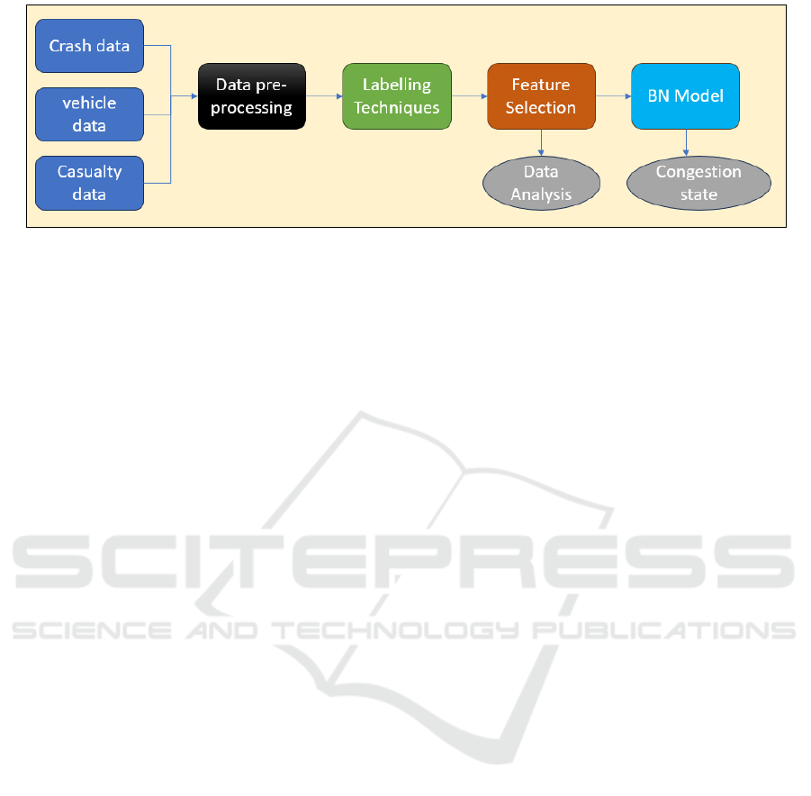
Figure 1: Block diagram of complete workﬂow of Trafﬁc congestion Analysis and Prediction.

non-recurring type congestion challenging to manage

and mitigate. It involves dynamic management and

immediate response to speciﬁc incidents to control

non-recurring congestion (Afrin and Yodo, 2021).

In the past, few attempts were made by researchers

to deﬁne the relation between congestion and road ac-

cidents (Zhang et al., 2019). Accidents occurring on

different road types signiﬁcantly impact congestion,

where the roadways are typically classiﬁed into ur-

ban, rural, and highways. Signiﬁcant congestion can

be caused due to the delay in response time by the

police or ambulance. In (Dias et al., 2009), vehicles’

speed is reduced during congestion, further reducing

the probability of accident occurrence. It’s important

to note that vehicles moving at high density during

congestion might lead to rear-end and side collisions.

This paper proposes a probabilistic Bayesian net-

work modeling for analyzing and predicting trafﬁc

congestion. The major objectives of this paper are:

• Building a Bayesian model for classifying the

congestion and identifying the root cause.

• Introducing novel congestion labeling criteria,

namely formula-based and hot spot-based ap-

proaches.

• Analysing the repetitive accident pattern causing

trafﬁc congestion.

• Evaluating and comparing the performance of the

proposed model with various machine learning al-

gorithms.

The remaining paper is organized as follows: Sec-

tion 2 explains the previous works on trafﬁc conges-

tion prediction. Sections 3 and 4 illustrate the label-

ing techniques and data pre-processing. The formal

introduction to Bayesian network and BN modeling

is described in Section 5. Furthermore, sections 6 and

7 consist of the analysis, results, and discussions, fol-

lowed by a conclusion in the ﬁnal section.

2 RELATED WORK

Over the past decade, researchers have tackled vari-

ous trafﬁc congestion problems, including trafﬁc con-

gestion prediction, trafﬁc demand analysis, better re-

routing to avoid congestion, accident prediction, ac-

cident duration estimation, etc. Some of the previous

works are detailed in this section.

In this paper (Gupta et al., 2022), the authors an-

alyzed the accident hotspots to understand the occur-

rence of severity at the danger zone using the Ker-

nal density estimator (KDE). Later, machine learn-

ing algorithms were used to determine the inﬂuencing

factors causing the accident’s severity. The best per-

formance was achieved using a sampling technique

named SMOTE and Random Forest. The authors

in (Zeng et al., 2016) developed a congestion factor

to identify the abnormal hotspots in a region. The

correlation between trafﬁc data and congestion fac-

tors was analyzed with the help of GPS data obtained

from taxis in China. This analysis helped to re-route

and manage trafﬁc when abnormal hotspots occurred.

In (Afrin and Yodo, 2021), the authors proposed a

Bayesian network to analyze the impact of variables

on congestion. The author implemented two BN mod-

els for recurring and non-recurring congestion in this

paper. Information like accidents and special events

was used to model the Bayesian network in a non-

recurring way. Furthermore, qualitative and quanti-

tative analysis was performed using both models to

provide a vision of the speed and number of vehicles

leading to congestion levels.

In (Ji et al., 2022), the authors proposed a free

model consisting of a digital and physical road net-

work. The digital twin network was the simulated

version of the physical road network. The digital twin

network was used to observe the trafﬁc and vehicle in-

formation, whereas Conv-LSTM was used to extract

spatio-temporal features from the physical network.

Both data sets were combined and processed to pre-

VEHITS 2024 - 10th International Conference on Vehicle Technology and Intelligent Transport Systems

dict congestion during an accident. Incident clearance

time has a direct impact on congestion. The authors

in (Ma et al., 2017) proposed a novel approach, Gra-

dient boosting decision tree(GBDTs), to predict the

duration of clearance time. It identiﬁes the complex

relationship between variables to shorten the clear-

ance time of the accidents. The authors in (Zhang

et al., 2019) used nine features, such as trafﬁc, acci-

dents, and environment features, to build two multi-

ple linear models—one to predict the clearance time

and the other for accident duration. The analysis il-

lustrated that accident duration was mainly impacted

by trafﬁc, road, and type of accident, whereas clear-

ance time depends on response duration and type of

accident. Results indicated that multiple linear regres-

sion models had outperformed the ANN model. In

(Santos et al., 2021), the authors proposed a predic-

tive model for predicting the occurrence of accidents

in the future based on historical data. Various super-

vised and unsupervised models were used to predict

the accident hotspots. A random forest model was

suggested to predict future accident hotspots better.

In (Chang et al., 2022), the authors explored con-

gestion and accident-prone regions by incorporating

a framework to extract relevant information from the

microblogs posted on social media platforms using

the NLP process and deep learning methods. Then,

a modiﬁed KDE technique was applied to identify the

prone regions, and data analysis was performed to pri-

oritize mitigating congestion and accidents.

Even though previous works used Bayesian net-

works in congestion analysis, mainly recurring and

non-recurring congestion, the use of accident infor-

mation is limited. In existing approaches, accidents

are considered one of many variables in modeling

non-recurring congestion. Using the broad spectrum

of variables related to accidents helps capture the

complexity of trafﬁc congestion accurately. Address-

ing the limitations, the uniqueness of our approach is

that we use many accident-related variables in deﬁn-

ing congestion. It also gives an in-depth insight into

the multifaceted nature of accidents and their impact

on road trafﬁc ﬂow. Our research introduces an inno-

vative labeling approach utilizing the extensive acci-

dent data in modeling Bayesian networks to forecast

the congestion level and identify variables that cause

congestion.

3 LABELLING TECHNIQUES

FOR CONGESTION

In this section, two labeling approaches are the for-

mula and hotspot approaches used for labeling the

congestion state. Both approaches are further cate-

gorized into 3-class and 2-class based on congestion

state.

3.1 Formula Based Approach

This approach creates a formula using the variables

available in the dataset. It is essential to consider

speed limit, severity, and number of cars involved in

an accident while determining trafﬁc congestion prob-

ability. The reason for considering these three vari-

ables more than others is as follows:

1. Number of Cars Involved. It provides informa-

tion about the number of vehicles involved in an

accident, which helps estimate the seriousness of

the incident. Accidents involving many vehicles

could be more severe, leading to delays, high con-

gestion, and a long time to clear the accident spot.

2. Severity. It helps assess the seriousness of the in-

cident and how much loss or damage it could have

caused based on fatalities, level of injuries, and

vehicle damages. There could be road blockage,

diversions, and high congestion when the severity

of an accident is high, as it might need fast medi-

cal emergency, investigation, and clearance.

3. Speed Limit. This variable shows the maximum

speed allowed on a particular road where an acci-

dent occurred. The consequence could be worse if

the accident happened on a road with a high-speed

limit, like highways, as it could cause delays for

authorities to reach the spot and clear it, leading

to increased congestion.

Using a heuristic approach, the congestion prob-

ability (CP) is formulated using the above three vari-

ables as shown in the equation 1.

The motivation for deﬁning equation 1 is based on

the widely accepted metric called Speed Performance

Index (SPI), a well-recognized concept used in trafﬁc

ﬂow assessment. SPI is described as the ratio of actual

vehicle speed and permissible maximum speed (road

speed limit), which can be utilized in classifying the

trafﬁc state as discussed in (Afrin and Yodo, 2021). In

our work, the speed limit variable is used similarly to

how it was used in calculating SPI, with slight modi-

ﬁcations. Equation 1 emphasizes the physical process

of disruption in trafﬁc ﬂow due to accidents. Incor-

porating features like severity, number of vehicles in-

volved in accidents, and speed limit helps to capture

the multifaced nature of trafﬁc congestion efﬁciently.

Below is the explanation of the equation in detail.

CP = 5 + 95 ·tanh



2(N + S

)

√

V + 1

·log

(N + 1)



(1)

Bayesian Network for Analysis and Prediction of Trafﬁc Congestion Using the Accident Data

Where N is the number of cars involved, S is the

severity of the accident, and V is the maximum speed

limit allowed on the road.

The S and N are combined, where S is squared

to give more weightage while calculating CP because

the severity level signiﬁcantly impacts congestion and

the spot’s clearance time. In the denominator, as the

value range of the speed limit V, which in its order

of magnitude is far higher than S and N, is applied

to compensate for it, the square root is used over V.

Then, the log ensures that the complexity factor in-

creases in a logarithmic way with the number of vehi-

cles involved in the collision. To bring the congestion

probability in the required range of [-1, 1], the tan-

gent function tanh(x) is used in the equation. The ﬁnal

output is shifted and scaled to ensure the probability

0 <= p <= 1.

3.1.1 3-Class Model

After obtaining the congestion probability from the

above-derived equation 1, we deﬁne the congestion

variable (target label) and categorize it into three

states representing the three classes of interest: low,

medium, and high. The labeling for congestion clas-

siﬁcation is performed based on speciﬁc criteria, in-

cluding type of road (rural, urban, and highway), level

of accident severity, and number of cars involved in

the accidents. Below is the criteria ﬂow chart and its

conditions:

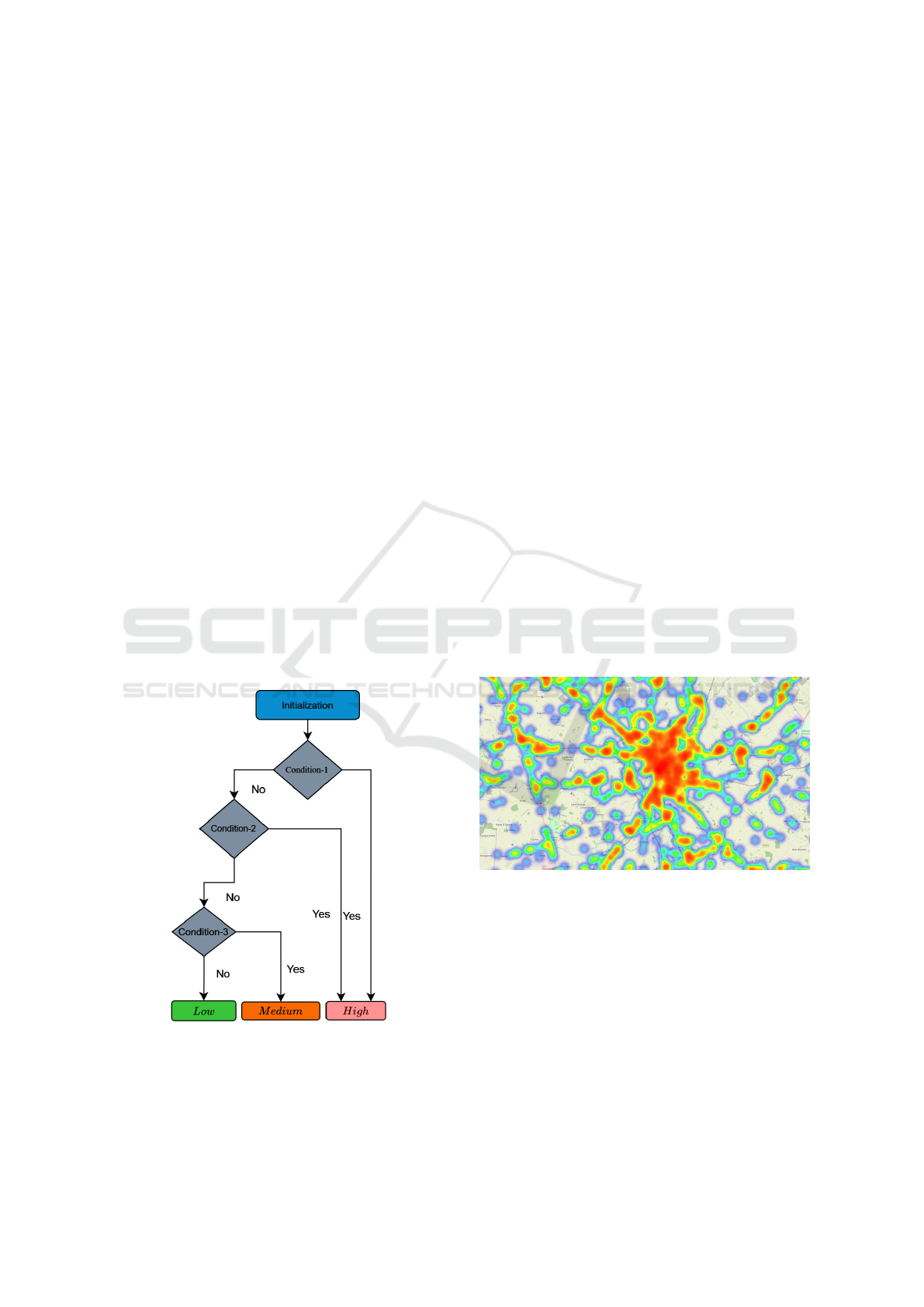
Figure 2: Flow chart for 3-class classiﬁcation using

formula-based approach.

In the below conditions, Road

Cat

, Low

, High

indicates road category, lower, and higher threshold

respectively.

• Initialization: Low

= 50, High

= 80

• Condition-1: N >= 3 OR CP = High

• Condition-2: Road

Cat

= (Urban OR Rural) AND

S = (Fatal OR Serious)

• Condition-3: CP > Low

AND Road

Cat

Urban AND S = Slight

3.1.2 2-Class Model

Similarly, this section deﬁnes the congestion variable

and categorizes it into low and high classes. The same

approach as above is being used. This 2-class classiﬁ-

cation is performed to observe the effect of the classi-

ﬁcation state on the performance of the proposed BN

model.

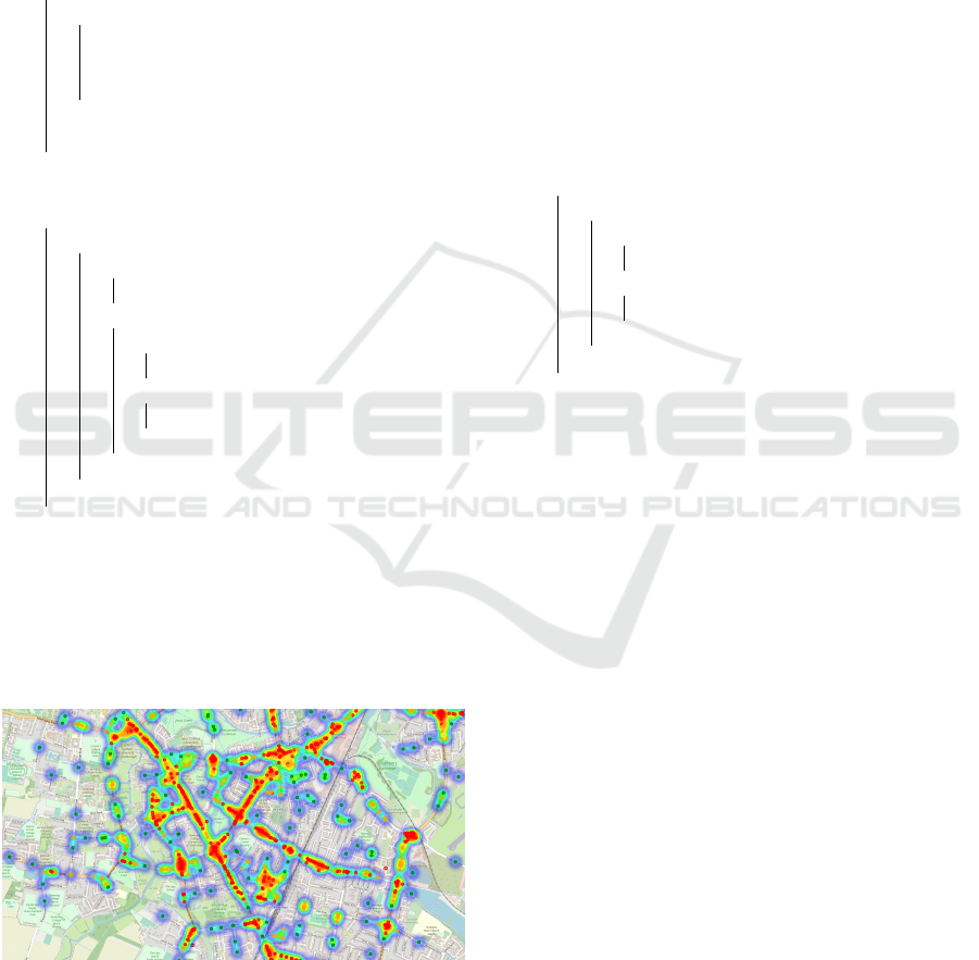
3.2 Hotspot Based Approach

This approach generates the hotspots based on the

number of accidents in a particular area. The accident

coordinates are provided in the dataset to identify the

location of the accident. Using those values, we can

plot on the map and see where hotspots are found, as

shown in Figure 3. Identical to the formula-based ap-

proach, the hotspots are categorized into 3-class and

2-class. Their entire process of classiﬁcation is illus-

trated in the below subsections.

Figure 3: Plotting all accident locations of Cambridgeshire.

3.2.1 3-Class Model

In this section, a heat map is created for the region of

Cambridgeshire to visualize geographical data, i.e.,

latitude (lat) and longitude (lon) points, and calcu-

late the number of accidents that occurred within the

given radius of each data point using geospatial anal-

ysis. The estimated number of accidents is then used

to ﬁnd the congestion state (congestion level), namely

low, medium, or high, as shown in Figure 4. This

algorithm consists of two functions: the NearbyAc-

cident function gives the number of accidents within

VEHITS 2024 - 10th International Conference on Vehicle Technology and Intelligent Transport Systems

the radius = 100 meters stored in the NearbyCount

variable, and the CongestionLevel function classiﬁes

the labels into three states. The complete process is

clearly shown in the Algorithm 1.

Data: Road accident data with lat, lon

Result: Congestion levels: low, medium, or

high

Function NearbyAccident(dataframe,

Radius):

for rows in dataframe do

Get lat, lon of accident;

Calculate distance to all points in

dataframe using Haversine formula;

end

return NearbyCount;

return

Function

CongestionLevel(NearbyCount):

for rows in NearbyCount do

if NearbyCount < 3 then

return low;

else

if NearbyCount < 6 then

return medium;

else

return high;

end

return

Initialization: Radius;

CALL NearbyAccident(dataframe,

Radius) ;

CALL CongestionLevel(NearbyCount) ;

Algorithm 1: Algorithm for 3 class congestion.

Figure 4: Mapping of color based on hotspot for congestion

level.

3.2.2 2-Class Model

The heat map creation is similar to the 3-Class model

except that classiﬁcation is only done in two states:

low and high. The congestion level is calculated using

Algorithm 2, shown below. Congestion is considered

low if the accident count with a given radius is less

than four, or else it’s considered high. A balanced

dataset requires a threshold of number of accidents

< 4 because an increase in the count would cause bi-

asing towards one of the congestion categories while

affecting the model performance.

Data: NearbyCount - a count of nearby

elements

Result: Congestion level: low or high

Function

CongestionLevel(NearbyCount):

for rows in NearbyCount do

if NearbyCount < 4 then

return low;

else

return high;

end

return

Algorithm 2: Algorithm for 2 class congestion.

4 DATA PRE-PROCESSING

4.1 Dataset

The dataset contains information about trafﬁc col-

lisions in Cambridgeshire (Cambridgeshire County

Council, 2018). This data is collected from 1st Jan

2017 to 31st July 2023, with speciﬁc criteria data in-

cluded. To include the data, it should be ofﬁcially

reported to the police with at least one person being

injured. Furthermore, at least one vehicle should have

been involved in the crash.

The dataset is split into three parts: Crashes, Ve-

hicles, and Casualties. The crash data contains all the

information about the trafﬁc, weather, and other vari-

ables related to the collision. The features involving

information about the vehicle, such as vehicle type,

vehicle maneuver, vehicle ﬁrst point of impact, etc.,

are placed in the Vehicle data sheet. The casualty

data is related to the injured person: casualty age, sex,

severity, etc.

’Collision Reference No.’ is the unique column

in all three data sheets, which helps correlate the data

across the data sheets. Furthermore, this correlated

Bayesian Network for Analysis and Prediction of Trafﬁc Congestion Using the Accident Data

data gives a detailed overview of each accident, which

helps analyze the data from the perspective of conges-

tion patterns.

4.2 Variables Discretization

The dataset consists of many variables, but from each

dataset, only certain variables are considered based on

the assumption that these variables could contribute

more to the congestion analysis. Therefore, we se-

lected from the datasets the following variables: char-

acteristic for crash - in Table 1; for casualty - in Ta-

ble 2; for vehicle - in Table 3. Furthermore, all the

used variables consist of discrete states. One major

problem during data pre-processing is inappropriate

distribution across the various variable states. Hence,

two steps are carried out. In step 1, we limit the vari-

able states; possible states are combined into a sin-

gle state, providing a meaningful state name. In an-

other step, a new state, ”Others” is created for some

variables to combine the number of categories con-

taining a limited amount of data in each state. For

instance, the weather variable consists of seven dis-

crete states: ”Fine with high winds, Fine without

high winds, Raining with high winds, Raining with-

out high winds, Snowing with high winds, Snowing

without high winds, Fog or mist - if hazard”.

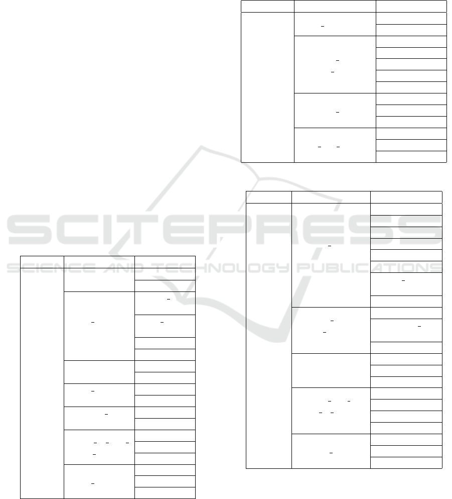
Table 1: Variables of the Crash dataset and their states.

Type Variable name States

Crashes

Day

Weekday

Weekend

Road Type

Single

carriageway

Dual

carriageway

Roundabout

Others

Weather

Good

Bad

Road

Conditions

Wet

Dry

Lighting

Conditions

Dark

Daylight

Types of turn

being made

Right turn

Left turn

No turn

Time period

PM Peak

AM Peak

OFF Peak

As the data across each state is deﬁcient, it is con-

verted into two states: good (Fine with high winds,

Fine without high winds) and bad ( Raining with high

winds, Raining without high winds, Snowing with

high winds, Snowing without high winds, Fog or mist

- if hazard). So accordingly, all the variables are pre-

processed, and the variables, along with their states,

are given in Tables 1, 2, and 3.

Table 2: Variables of Casualty dataset and their states.

Type Variable name States

Casualties

Num Casualties

low

high

Casualty

Vehicle group

Pedal Cycle

Car

Motorcycle

Pedestrian

Others

Casualty severity

Slight

Serious

Fatal

Seat belt used

Worn

Not applicable

Others

Table 3: Variables of Vehicles dataset and their states.

Type Variable name States

Vehicles

Vehicle

Manoeuvre

Slowing

L-Bend Ahead

Moving off

Turning right

R-Bend Ahead

Turning left

Going

ahead other

Others

Alcohol

breath test

Negative

Driver not

contacted

Others

Skidding

No skidding

Skidded

Flipped

Vehicle ﬁrst

point of

impact

Nearside

Offside

Front

Others

Journey purpose

Work trip

Not Known

Others

VEHITS 2024 - 10th International Conference on Vehicle Technology and Intelligent Transport Systems

5 IMPLEMENTING A BAYESIAN

NETWORK FOR TRAFFIC

CONGESTION

5.1 Bayesian Network

The Bayesian network is a probabilistic graphical

model that uses a direct acyclic graph(DAG) approach

to represent the conditional dependencies between the

variables. This model is robust in tackling uncertain-

ties and can capture complex hidden relationships be-

tween sets of variables. It is used in various domains

like road trafﬁc management, health care, etc. These

Bayesian networks are also called Bayes networks or

Belief networks (Nagarajan et al., 2013).

5.1.1 Fundamental Features of BN

• Nodes and Edges. In a Bayesian network, nodes

represent variables or features. There are various

types of nodes, such as discrete, continuous, etc.,

whereas Edges or arrows deﬁne the strength of the

conditional relationship between those variables.

• Conditional Independence. One of the most crit-

ical characteristics of the Bayesian network is that

it can represent the conditional independence be-

tween the variables. For instance, if two nodes

are conditionally independent, knowing the state

information of one node doesn’t provide any in-

formation on the state of the other node, given

the parent node state is known. This character-

istic helps to simplify the model when there is a

complex relationship.

• Joint Probability Distribution. A Bayesian net-

work can compactly represent a set of variables’

probability distribution. Let’s say X1, X2, . . . Xn

are the network variables; joint probability dis-

tribution can be deﬁned as the product of each

node’s conditional probability provided by its par-

ent node (Kjaerulff and Madsen, 2008).

P(X

, X

, . . . , X

) =

∏

i=1

P(X

| Parents(X

)) (2)

5.1.2 Formulas and Calculation

• Bayes’ Theorem. The fundamental principle of

Bayesian networks helps update the probability of

the hypothesis when more information is provided

as evidence (Kjaerulff and Madsen, 2008). The

mathematical representation of Bayes’therorem

is:

P(A | B) =

P(B | A) ×P(A)

P(B)

(3)

Where: P(A|B) is the probability of the occur-

rence of event A, given that some evidence on B.

It is called posterior probability. P(B|A) is the

probability of the occurrence of event B, given

that A is true. P(A), P(B) are the probability of

occurrence of event A and B. These are also called

prior probabilities.

• Inference in BN. This is the process of calcu-

lating the posterior probability of an event when

given evidence on other variables. The Inference

in the Bayesian Network is also utilized in diag-

nosis or predictions based on uncertain or incom-

plete information.

• Learning in BN. The Bayesian networks can

compute the conditional probabilities table (CPT)

from the data using methods like EM estimator

or maximum likelihood estimator (Yang et al.,

2019).

5.2 BN Structure

The proposed structure of the Bayesian Network con-

sists of 17 variables, which are taken from three dif-

ferent data sheets as described in section 5.2. The de-

sign of the BN is performed with the help of Random

Forest to gather the importance of the features and the

structure learned from the data by using the HUGIN.

The model is built based on these approaches. The

model shown in Figure 5 is used for classiﬁcation.

The formula and hotspot-based approach are used

only for data labeling. Another model is used where

the BN model’s structure and parameters are learned

from the data. This model is used as a base model,

which will be helpful when comparing the perfor-

mance of the proposed model.

5.3 Evaluation Metrics

The confusion matrix is used to evaluate the model

performance in classiﬁcation tasks. It gives infor-

mation about the actual and model-predicted classes.

True Positive, True Negative, False Positive, and

False Negative are the four essential elements in the

confusion matrix that can be used to calculate met-

rics like Accuracy, Precision, Recall, and F1-score to

assess the model’s performance.

6 DATA ANALYSIS

This section is divided into data visualization for an-

alyzing the correlation patterns between the features

Bayesian Network for Analysis and Prediction of Trafﬁc Congestion Using the Accident Data

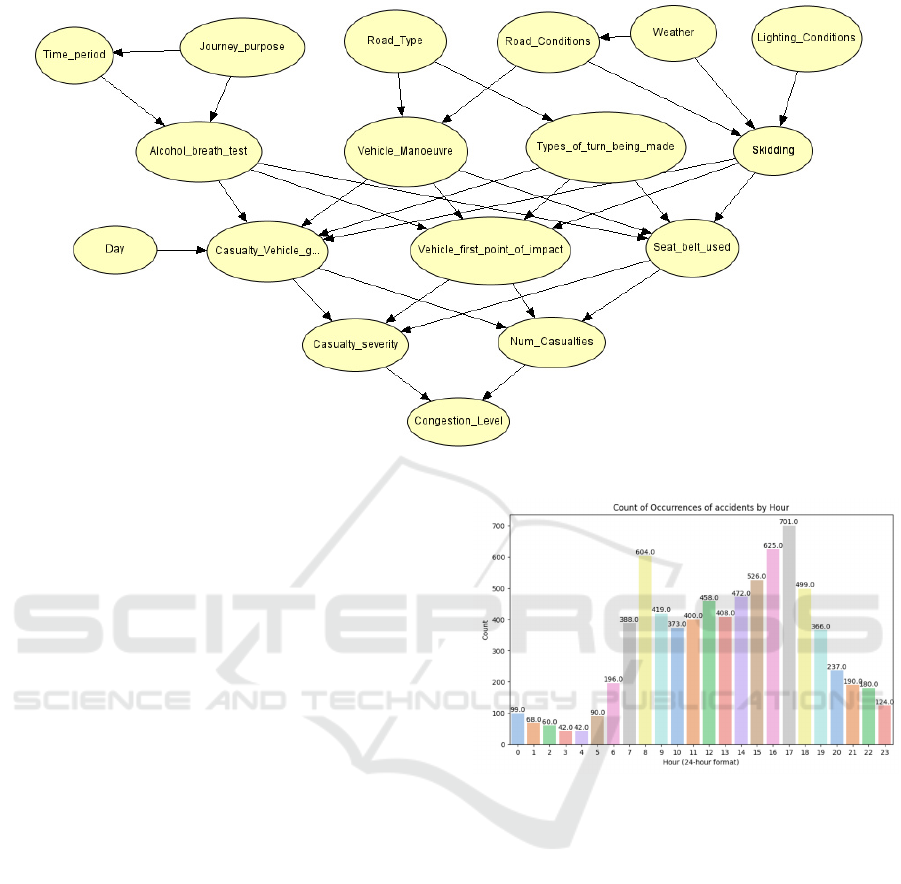
Figure 5: Diagram of Proposed Bayesian Network.

and scenarios for diagnosis and predictive analysis of

the Bayesian Network.

6.1 Data Visualization

The bar plot shown in Figure 6 shows the occurrence

of road accidents by hour in Cambridgeshire. There

is a signiﬁcant rise in accidents in the late afternoon,

around 16:00 to 18:00, and most accidents, i.e., 701

cases, occurred at 17:00, which can be observed from

Figure 6. Another prominent rise can be observed

during morning rush hour at 8:00 when people usu-

ally go to the ofﬁce or school. The data shows that

most accidents occurred more frequently during rush

hour. These accident patterns are correlated to peak

hours of trafﬁc congestion patterns. So, a trafﬁc man-

agement system should address trafﬁc congestion to

reduce accidents.

The relationship between congestion probability

and accident severity is illustrated using the violin

plot in Figure 7. The severity is categorized into

slight, severe, and fatal, and data is plotted based on

these severity types. This wider violin shape in the

plot indicates that congestion probability is high for

that severity type.

From Figure 7, it is evident that the relationship

between the severity causes the congestion. With the

increase in severity, the probability of congestion also

increases. The data distribution also states that slight

severity has a lesser impact on congestion when com-

pared with Serious and fatal accidents. Moreover, all

the Figures 7, 8, 9 use equation 1 for the computation

of the congestion probability on the y-axis.

Figure 6: Number of road accidents happened on an Hourly

basis.

The plot in Figure 8 illustrates the number of ve-

hicles involved, leading to congestion probability on

different road types. From Figure 8, it is clear that,

with the number of vehicles, the congestion proba-

bility rises across all the road types, which indicates

that more vehicles are likely to cause more conges-

tion. The data distribution shows that, for urban roads,

there is a steep rise in congestion with fewer vehicles

involved. In contrast, there is a moderate rise in con-

gestion probability on rural roads and highways. So,

the distribution implies that urban roads are more sen-

sitive to vehicle accidents.

Figure 9 describes the congestion probability

based on accident severity across different road types.

The trend shows that, despite road type, the likelihood

of congestion increases with the increase in severity.

For instance, fatal accidents for all road types cause

VEHITS 2024 - 10th International Conference on Vehicle Technology and Intelligent Transport Systems

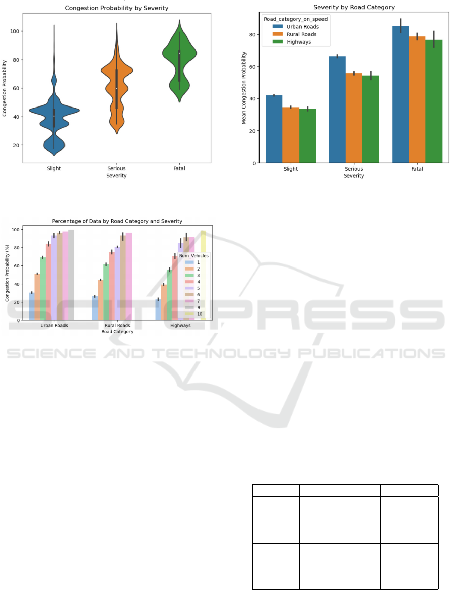
Figure 7: A plot of level of severity impacting the conges-

tion probability.

Figure 8: Plot for the effect of number of vehicles involved

in an accident over congestion probability.

a higher impact on congestion. And from the data,

urban roads exhibit more congestion when compared

to rural roads and highways for all levels of sever-

ity. This is because the volume of trafﬁc on urban

roads and complex trafﬁc dynamics are higher. So, to

address trafﬁc congestion, the strategies should also

consider severity and road type.

6.2 Scenarios Evaluation

From the accident dataset, the probability distribution

for each variable obtained deﬁnes the default proba-

bilities of the BN model. People tend to go to the

ofﬁce and school in the AM peak mornings and re-

turn PM peak in the evenings, mainly on weekdays.

The accident dataset shows a 77.57% likelihood for

accidents during the weekdays, whereas 22.43% on

weekends. Following a similar trend, the probability

of time period is 38.47%, 42.09%, and 19.44% for

AM, PM, and OFF peaks, respectively. The probabil-

ity of good weather is 84.15%, and 71.63% of road

conditions are dry. So, it is less likely that the vehicle

will skid. Hence, as per the dataset, the chances of no

Figure 9: Bar plot to indicate the data distribution based on

road category and severity.

skidding are higher at 79.73%, while vehicle skidding

and ﬂipping are very low.

As most of them are car users, with a likelihood of

47.15%, and wearing the seat belt, there is a chance

of slight severity to the person, with a probability of

72.88%, which leads to further reducing the number

of casualties to 72.87%. Combining the states of num-

ber of casualties and casualty severity, the probabil-

ity of congestion level being low is 28.98%, medium

is 35.44%, and high is 35.58%. The likelihood of

medium and high are almost the same from the data.

Apart from default probabilities as detailed above,

six different scenarios are created to observe the im-

portance of variables and probability distribution of

variables that cause congestion. All these scenarios

are classiﬁed correctly with the proposed BN model,

as shown in Figure 10. A 2-class congestion state ex-

plains scenarios 1 and 2, whereas the remaining four

scenarios are demonstrated using a 3-class congestion

state.

Table 4: Probability distribution of congestion state based

on scenario 1 and 2.

Scenario Variable (state) Congestion

Alcohol test

(negative) &

Casualty severtiy

(low)

Low

(77.78%)

Alcohol test

(positive) &

Casualty severtiy

(serious)

High

(74.24%)

Scenario-1, 2 were created for varying the Alco-

hol breath test and casualty severity for 2-class con-

gestion state as shown in Table 4. In scenario 1, the

Bayesian Network for Analysis and Prediction of Trafﬁc Congestion Using the Accident Data

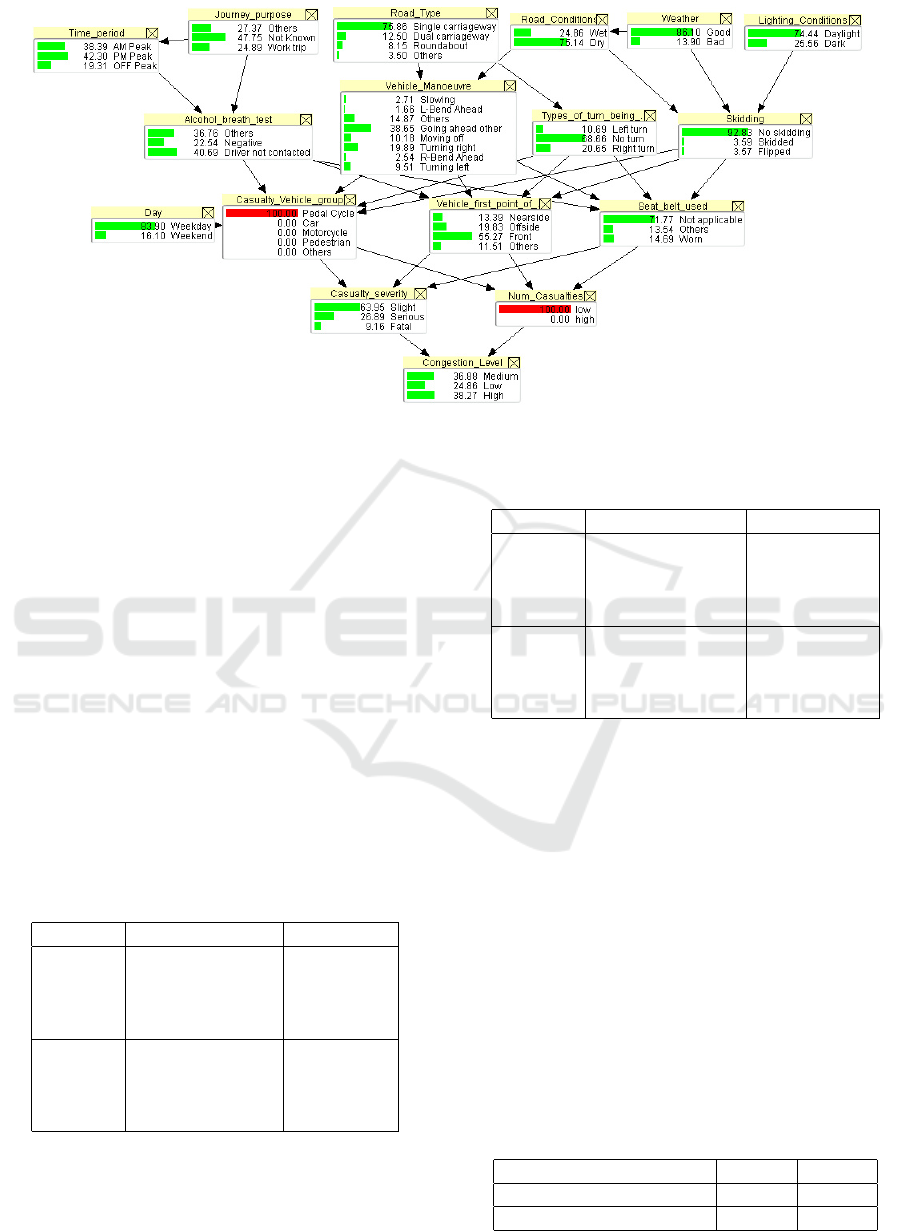
Figure 10: Diagram of Bayesian Network with evidence for Scenario-3, 4.

alcohol test is negative, and casualty severity is slight.

A low level of congestion is being observed with a

probability of 77.78%. Scenario 2 consists of the al-

cohol test state as positive (it is a part of the Others

category), and severity as serious, and the 74.24%

congestion level is higher. Here, the seriousness of

the accidents inﬂuences the impact on congestion.

Scenario-3, 4. These are created to vary the casu-

alty vehicle group and number of casualties to show

the impact of the vehicle group are shown in Table 5.

In scenario 3, one of the casualty vehicle group states

is pedestrian and has a low number of casualties; then,

the likelihood of congestion is medium, with 39.42%.

In scenario 4, the Pedal cycle is the state of vehicle

group type with a low number of casualties, and then

there is a 38.27% chance of congestion being high as

shown in Figure 10.

Table 5: Probability distribution of congestion state based

on scenario 3 and 4.

Scenario Variable (state) Congestion

Casualty veh grp

(pedestrian) &

Num of casualty

(low)

Medium

(39.42%)

Casualty veh grp

(Pedal cycle) &

Num of casualty

(low)

High

(38.27%)

Scenario-5, 6: are created to vary the casualty

severity and the number of casualties as shown in Ta-

ble 6. In scenario 5, with slight casualty severity and

low casualties, the congestion probability is medium,

with a probability of 55.75%. In scenario 6, when the

Table 6: Probability distribution of congestion state based

on scenario 5 and 6.

Scenario Variable (state) Congestion

Casualty severity

(slight) &

Num of casualty

(low)

Medium

(55.75%)

Casualty severity

(serious, fatal) &

Num of casualty

(high)

High

(91.7, 99.1%)

number of casualties is high with the severity of casu-

alty as serious and fatal, then congestion probability

is high at 91.17% and 99.1%, respectively.

7 RESULTS AND DISCUSSION

Table 7 illustrates the accuracy of two labeling ap-

proaches for different classes. From the table, it is

clear that formula-based approaches have better per-

formance when compared with the hotspots-based ap-

proach, which gives model accuracy of 45% and 52%

for 3-class, 2 class respectively. One of the main rea-

sons for the lower performance is the variables used

for labeling.

Table 7: Performance of proposed model using both ap-

proaches.

3-class 2-class

Formula Based approach 0.66 0.89

Hotspot Based approach 0.45 0.52

VEHITS 2024 - 10th International Conference on Vehicle Technology and Intelligent Transport Systems

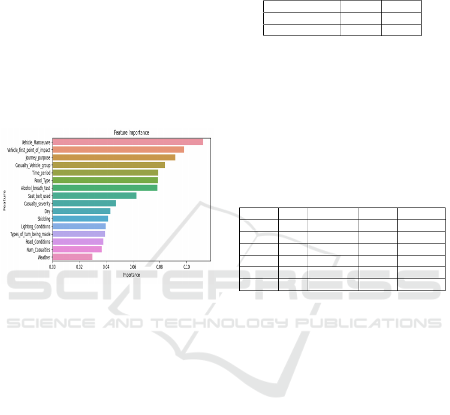
In the hotspot approach, only the geographical co-

ordinates of the accidents were used based on the

number of accidents deﬁned in that hotspot region.

Because of this, the dataset’s features did not con-

tribute to the target congestion label, as shown in Fig-

ure 11.

This ﬁgure 11 shows the feature importance gen-

erated using the Random forest. It is evident that

the variables contribute less to the target (congestion

state). Even though the vehicle maneuver has the

highest importance, it contributes only 0.1 to the clas-

siﬁcation of the congestion state. Hence, the hotspot

labeling approach performance is deﬁcient.

Figure 11: Feature importance for a hotspot-based approach

using Random Forest.

On the other hand, using the formula-based ap-

proach, model accuracy with 2-class (congestion

states are low and high) is 89%, while the 3-class

model accuracy is 66%. The low performance of the

model in 3-class variations is due to the lack of data.

The Bayesian model was trained on only 6000 records

of accidents from 6 years with certain criteria. As the

data is low, the proposed BN model performance is

affected.

The table 8 explains the performance of the pro-

posed model compared to the Base model. The pro-

posed model with hotspot labeling is used for the

comparison as the performance difference of the Base

model is signiﬁcantly higher than the hotspot ap-

proach. In contrast, for the formula-based approach,

the model performance is slightly superior to the Base

model. In the proposed model, the structure of the

model is deﬁned, and the parameters of the model are

learned from the data. In contrast, in the Base model,

both the structure and the parameters are learned from

the data. Even though the base model performance

is high, the complexity is extremely high simultane-

ously.

The Base model has generated many casualty re-

lationships between variables, drastically increasing

Table 8: Comparison of model performance between Pro-

posed model and Base model.

3-class 2-class

Proposed Model 0.45 0.52

Base Model 0.58 0.71

the conditional probability table (CPT) order. As the

complexity of the model rises, it takes longer training

time and requires higher computational resources. So,

there is also a need to look for the trade-off between

model performance and complexity.

Table 9 illustrates the performance of the proposed

Bayesian Network (BN) model for 2-class and is com-

pared with different machine learning models, namely

Logistic regression (LR), Decision Tree (DT), Ran-

dom Forest (RF), Support Vector Machine (SVM),

and K-Nearest Neighbor (K-NN).

Table 9: Comparison of Proposed model performance

against ﬁve different Machine learning models.

Model Acc Precision Recall F1-score

LR 0.88 0.87 0.98 0.92

DT 0.83 0.89 0.86 0.88

RF 0.87 0.87 0.95 0.91

SVM 0.88 0.87 0.98 0.92

K-NN 0.82 0.83 0.93 0.88

BN 0.89 0.90 0.72 0.81

All the models are computed on the same data,

split into an 80:20 ratio. All the models were trained

on 80% of the data, and the remaining 20% was used

to evaluate the model. The results are shown in ta-

ble 9. From the results, the accuracy of the proposed

BN model is slightly outperforming the other machine

learning models. The proposed model’s accuracy is

89%, while LR and SVM are closer, with an accuracy

of 88%. The proposed model is also outperforming

with 90% precision, while DT has a more intimate

precision of 89%. The evaluation metrics Recall and

F1-score are low for the proposed model, with 72%

and 81%, respectively.

To summarize the results, the proposed Bayesian

Network has shown competitive performance com-

pared to the above machine learning models. More-

over, as Bayesian Networks are probabilistic graphi-

cal structured models, they can provide interpretation

of results and explainability. It can be used to model

the causal relationship between trafﬁc variables and

is also good at handling uncertainty. These qualities

of the Bayesian network offer an advantage in debug-

ging the root cause of trafﬁc congestion and road ac-

cidents.

Bayesian Network for Analysis and Prediction of Trafﬁc Congestion Using the Accident Data

8 CONCLUSION

This paper proposes a Bayesian Network that uses ac-

cident data analysis to label and predict congestion

states. There are various approaches to deﬁne conges-

tion from accident datasets. In this work, a novel tech-

nique for labeling congestions uses formula-based

and hotspot-based approaches. Furthermore, to ob-

serve the model performance, the congestion states

were classiﬁed into 3-class states (low, medium, and

high) and 2-class states (low, high). The results

show that the proposed model performance is higher

in 2-class predictions, especially with the formula-

based approach of 89.1% accuracy compared to the

hotspot approach. This is the novelty of our ap-

proach. This performance is compared with differ-

ent machine learning models (Random Forest, Deci-

sion Tree, SVM, Logistic Regression), which show

that the proposed model has slightly better accuracy

and precision. It also demonstrated comparable per-

formance with ML models.

The main limitation of this work is that we re-

strict our focus to accident information. Even though

it provides valuable insights, it does not consider all

the other factors causing congestion. Moreover, we

acknowledge the need for further reﬁnement on a

hotspot-based approach to improve its performance,

and a dedicated Bayesian model needs to be imple-

mented. Further, we will build a Dynamic Bayesian

Network focusing on the hotspot approach to label

the congestion and follow its development trends. We

will also use various factors near the hotspot, like the

speed of other surrounding vehicles, junction type,

and other points of interest (Schools, Hospitals, etc.).

Besides accidents, future work will also focus on

the root causes of non-recurring congestion due to

unforeseen events, like construction works, weather-

related, and special events. Social media blogs and

platforms can provide further insights into accident

modeling. Moreover, it is also signiﬁcant to under-

stand the correlation between road safety measures,

congestion, and their joint impact on urban mobility.

REFERENCES

Afrin, T. and Yodo, N. (2021). A probabilistic estimation of

trafﬁc congestion using bayesian network. Measure-

ment, 174:109051.

Cambridgeshire County Council (2018). Cam-

bridgeshire road trafﬁc collision data. https:

//data.cambridgeshireinsight.org.uk/dataset/

cambridgeshire-road-trafﬁc-collision-data. Ac-

cessed: October 10, 2023.

Chang, H., Li, L., Huang, J., Zhang, Q., and Chin, K.-S.

(2022). Tracking trafﬁc congestion and accidents us-

ing social media data: A case study of shanghai. Ac-

cident Analysis & Prevention, 169:106618.

Dias, C., Miska, M., Kuwahara, M., and Warita, H. (2009).

Relationship between congestion and trafﬁc accidents

on expressways: an investigation with bayesian belief

networks. In Proceedings of 40th Annual Meeting of

Infrastructure Planning (JSCE), Japan.

Gupta, U., Varun, M., and Srinivasa, G. (2022). A compre-

hensive study of road trafﬁc accidents: Hotspot anal-

ysis and severity prediction using machine learning.

In 2022 IEEE Bombay Section Signature Conference

(IBSSC), pages 1–6. IEEE.

Ji, X., Yue, W., Li, C., Chen, Y., Xue, N., and Sha, Z.

(2022). Digital twin empowered model free predic-

tion of accident-induced congestion in urban road net-

works. In 2022 IEEE 95th Vehicular Technology

Conference:(VTC2022-Spring), pages 1–6. IEEE.

Kjaerulff, U. B. and Madsen, A. L. (2008). Bayesian net-

works and inﬂuence diagrams. Springer Science+

Business Media, 200:114.

Ma, X., Ding, C., Luan, S., Wang, Y., and Wang, Y.

(2017). Prioritizing inﬂuential factors for freeway

incident clearance time prediction using the gradient

boosting decision trees method. IEEE Transactions on

Intelligent Transportation Systems, 18(9):2303–2310.

Nagarajan, R., Scutari, M., and L

ebre, S. (2013). Bayesian

networks in r. Springer, 122:125–127.

Santos, D., Saias, J., Quaresma, P., and Nogueira, V. B.

(2021). Machine learning approaches to trafﬁc ac-

cident analysis and hotspot prediction. Computers,

10(12):157.

Wang, C. (2010). The relationship between trafﬁc conges-

tion and road accidents: an econometric approach us-

Yang, Y., Gao, X., Guo, Z., and Chen, D. (2019). Learning

bayesian networks using the constrained maximum a

posteriori probability method. Pattern Recognition,

91:123–134.

Zeng, L., Hu, X., Han, Q., Ye, L., Wang, R., He, X., and Xu,

Y. (2016). Abnormal hotspots detection method based

on region real-time congestion factor. In 2016 IEEE

19th International Conference on Intelligent Trans-

portation Systems (ITSC), pages 749–753. IEEE.

Zhang, J., Junhua, W., and Shou’en, F. (2019). Prediction of

urban expressway total trafﬁc accident duration based

on multiple linear regression and artiﬁcial neural net-

work. In 2019 5th International Conference on Trans-

portation Information and Safety (ICTIS), pages 503–

510. IEEE.

VEHITS 2024 - 10th International Conference on Vehicle Technology and Intelligent Transport Systems