GraphVault: A Temporal Graph Persistence Engine

Julian Bichl

1,2

, Thomas Driessen

, Melanie Langermeier

and Bernhard Bauer

qbilon GmbH, Hermanstraße 5, 86150 Augsburg, Germany

Software Methodologies for Distributed Systems, University of Augsburg,

Universitatstrasse 6a, 86135 Augsburg, Germany

Keywords:

GraphVault, Temporal Graphs, Graph Query Engine, Temporal Graph Persistence, Graph Databases.

Abstract:

Graph structures have gained increasing popularity in recent years as they offer comprehensive possibilities for

managing and analyzing high interconnected data. In order to facilitate the orchestration of these data, graph

databases have been developed enabling graphs to be stored as central entity. However, traditional graph

databases and frameworks consider graphs as a inherently valid unit without temporal reference which can

limit their ability to perform advanced analysis. This paper presents GraphVault, a graph persistence engine

that is capable of efﬁciently storing graphs and reconstructing labeled property graphs over time. We present

our temporal data model, which we mapped to a key-value engine using a purpose-built record design. The

performance of our implementation is then compared to that of a conventional graph database.

1 INTRODUCTION

At the beginning of the 21st century, technical ad-

vancements in Big Data enabled the capturing of

highly interconnected information, in which not only

the individual data record but the interconnectivity

of the data among each other serves as the main

source of knowledge acquirement. While common

data structures like tables are unsuitable for represent-

ing highly interconnected data, graphs consisting of

attributed nodes and edges provide a decisive capa-

bility in structuring and analyzing connected informa-

tion. Current research considers graphs as key enabler

for future advances, e.g. the Gartner Inc. predicts an

80 percent use of graphs and graph technologies in

shaping innovation by 2025 (Rita, 2021).

However, common graph database systems can

only store static graphs. Therefore, observing and an-

alyzing past graph mutations over time is not natively

supported by most systems. This missing informa-

tion represents enormous untapped potential. E.g. Fi-

nancial Fraud Detection uses graph databases to iden-

tify fraud rings through reused telephone numbers or

addresses (Sadowski and Rathle, 2014). Employing

a temporal graph database, such rings could also be

identiﬁed over time even if the fraudsters never used

identical data records at the same period of time. An-

other example of graph databases in action are prod-

uct recommendation systems enabling the generation

of targeted recommendations for customers by linking

products to their associated buyers. As customer buy-

ing behavior changes over time, the use of a temporal

graph database could weaken the evaluation quality

of past purchases or could incorporate seasonal events

into the generation of new product recommendations.

These examples demonstrate the potential advan-

tages of incorporating the temporal dimension into

existing graph databases. This paper introduces

GraphVault, a robust temporal graph persistence en-

gine that can efﬁciently store a graph over time and

rebuild it at any earlier point.

The remaining paper is structured as follows: In

Chapter 2 we give an overview over different exist-

ing approaches that enabled graph tracking over time.

Following this summary, our paper presents our solu-

tion in chapter 3, in which we have mapped a tem-

poral graph model to a key-value engine. Our ap-

proach is further evaluated in Chapter 4, where we

compare the query performance of past graphs to a

general used graph database.

2 RELATED WORK

In recent years, there have been several solutions to

connect temporal dimension with graph databases and

thereby track changes over time. The following chap-

ter provides an overview of the most relevant ap-

224

Bichl, J., Driessen, T., Langermeier, M. and Bauer, B.

GraphVault: A Temporal Graph Persistence Engine.

DOI: 10.5220/0012556500003690

Paper published under CC license (CC BY-NC-ND 4.0)

In Proceedings of the 26th International Conference on Enterprise Information Systems (ICEIS 2024) - Volume 1, pages 224-231

ISBN: 978-989-758-692-7; ISSN: 2184-4992

proaches. However, the list does not claim to be ex-

haustive and rather points out approaches that differ

signiﬁcantly from each other.

The approach presented by Massri et al. is based

on a columnar database and tries to optimize the cal-

culation time during querying the graph at a given

point in time, while minimizing the amount of storage

used to store graph mutations (Massri et al., 2020). In

their research they deﬁned the Copy Model (complete

graph snapshots are saved despite high redundancy),

the Log Model (only the initial graph and the changes

are saved) and the Copy-on Write Model (only mod-

iﬁed graph elements are copied). To achieve a com-

promise between the need of computational effort for

graph calcuation at a given point in time and neces-

sary storage to persist it, they introduced a new model

called Copy+Log. This model splits the graph history

into time chunks, which themselves are structured

by the Log Model with an initial graph and stored

graph mutations. Further development optimized the

querying time by implementing backwards calculable

graph modiﬁcations (Massri et al., 2023). This re-

duced the needed disk space by reducing the initial

graph to an amount of mutations applied on the initial

graph of the previous chunk.

Rost et al extended their distributed graph analy-

sis framework Gradoop in order to support temporal

validity for graph elements (Rost et al., 2019). By

adding two optional intervals to every record in their

columnar database, it was possible to attach the valid

and the transactional time to every node and edge.

On the basis of this additional information, they were

able to deﬁne temporal analysis operators executed on

their Apache Flink based processing engine. These

operators made it possible to query graphs at a given

time, to calculate the difference of two time-varying

graphs, to group graph elements with respect to the

temporal dimension and to check for graph patterns

considering temporal constraints.

The authors of ImmortalGraph developed an opti-

mized persistence method for temporal graphs in ad-

dition to a temporal graph processing engine (Miao

et al., 2015). Employing this approach, temporal

graph operators can be classiﬁed according to their

degree of temporal and structural complexity. The

graph data is duplicated stored and persisted in a

structure-local and temporal-local data structure.. To

efﬁciently perform computations on the graph struc-

ture at a certain point in time, the graph elements are

processed and persisted in a structure-local layout. If

one or more graph elements are considered over time,

the temporal-local layout is used to enable more efﬁ-

cient temporal operators.

Debrouvier et al. deﬁned a temporal property

graph model to extend a common graph database by

attaching validity intervals to the graph elements as

properties (Debrouvier et al., 2021). Less data re-

dundancy is achieved by decoupling property keys

and property values and internally representing them

as separated nodes. Their prototype is based on the

commercial graph database Neo4j. They further de-

veloped their graph query language T-GQL that trans-

lates into Cypher queries and were able to query dif-

ferent kinds of shortest paths over time.

3 GraphVault

In this chapter, we present GraphVault, a temporal

database system designed for efﬁcient graph persis-

tence over time and instant graph reconstruction from

any prior time point.

In the following, we use the deﬁnition proposed

in (Angles et al., 2017) as it provides the foundational

data structure for our improved temporal graph.

Deﬁnition 1.

A directed labeled property graph G is deﬁned as

G = (N, E, L, P,V, ε, λ, σ)

where

• N : {N

, ..., N

} is a set of nodes representing en-

tities identiﬁed by unique numeric IDs.

• E : {E

, ..., E

} is a set of directed edges repre-

senting relationships between nodes. Each di-

rected edge is identiﬁed by a unique numeric ID.

• L : {L

, ..., L

} is a set of labels assigned to nodes

and edges denoting the type or nature of the entity

or relationships. Labels are represented by string

values.

• P : {P

, ..., P

} is a set of properties identiﬁed by

a string.

• V : {V

, ...,V

} is a set of property values of any

datatype.

• ε : (ε

∪ ε

) is a set of functions with ε

: E → N

and ε

: E → N that maps every edge to a source

and target node.

• λ : (N ∪ E) −→ L is a total function that maps a

label to each node and edge.

• σ : (N ∪ E) ×P ↣ V is a injective partial function

that maps a node or a node with a property to a

corresponding property value.

■

This deﬁnition is frequently used as the funda-

mental data structure for common graph databases

GraphVault: A Temporal Graph Persistence Engine

225

and therefore yield to our data structure for our tem-

poral graph engine. In the academic literature, there

have been a number of different approaches to the

storage of graphs over time.

In their work, Salzberg and Tsotras introduced

the Copy and Log methods for temporal informa-

tion storage in graphs. Copy involves saving com-

plete graph states at each change, leading to redun-

dancy, while Log only records changes, reducing stor-

age but increasing reconstruction computational over-

head (Salzberg and Tsotras, 1999).

In order to avoid the need to store all snapshots

of the modiﬁcation of a graph or to compute all

modiﬁcations in order to regain the graph at a given

point in time, researchers used an alternative ap-

proach by assigning validity intervals to graph ele-

ments. This method is analogous to the expansion of

the SQL:2011 standard that included temporal func-

tionalities, where temporal intervals are assigned to

relational records (Kulkarni and Michels, 2012). Our

approach implemented in GraphVault is based on the

approach proposed by (Campos et al., 2016) and the

Duration-labeled temporal graph presented in (De-

brouvier et al., 2021), which assigns validity intervals

to nodes, edges, properties and property values.

Formally, our previously deﬁned labeled property

Graph G in Deﬁnition 1 is extended to:

Deﬁnition 2.

A temporal directed labeled property graph G

temporal

is deﬁned as

temporal

= (N, E, L , P,V, I, ε, λ, σ, ι)

where

• N, E, L, P,V, ε, λ, σ are deﬁned as in Deﬁnition 1

• σ : (N ∪ E) × P → {v

, ..., v

} ⊆ V is a function

that maps a node or an edge with a property to a

set of corresponding property values.

• I : {(a, b] | a, b ∈ N and a < b} As a set of validity

intervals, where a and b symbolize timestamps.

a is the ﬁrst timestamp where the corresponding

element was valid and b the point in time when

the element got invalid.

• ι : (N ∪ E ∪ P ∪V ) → {i

, ..., i

} ⊆ I is a function

that maps graph elements like nodes, edges, prop-

erties and property values to a subset of validity

intervals.

■

We also deﬁne some helper functions to better

specify the formal temporal graph model:

1. active : (N ∪ E ∪ P ∪V ) × N →Boolean

such that

active(e, i) =







True,

if ∃(a, b] ∈ ι(e) :

i ≥ a ∧ i < b

False, else

The function active indicates whether for a graph

element e at any point in time i the element ex-

isted.

These deﬁnitions allows us to attach validity in-

tervals to every graph element. There are additional

constraints enforced on the model, so that it remains

consistent and all graph states can be reconstructed at

any time in a valid state:

2. ∀i ∈ N, ∀e ∈ (N ∪E), ∀p ∈ P: σ(e, p) = v ∧v ̸=

active(i, v) ⇒ active(i, p)

This requirement guarantees that if a property

value existed at any point, the corresponding

property must have also been present.

3. ∀i ∈ N, ∀e ∈ (N ∪ E), p ∈ P : σ(e, p) ̸=

active(i, p) ⇒ active(i, e)

The same principle can be applied to nodes and

edges, as these must also be valid whenever an

associated property existed at that point in time.

4. ∀i ∈ N, ∀e ∈ E, n ∈ N : ε(e) = n,

active(i, e) ⇒ active(i, n)

The remaining constraint ensures that if an edge

existed at some time, the corresponding source

and target nodes must exist at that time.

These requirements ensure graph structure consis-

tency over time. However, additional rules must be

deﬁned to ensure the logical correctness of the graph

through time:

5. ∀e

, e

∈ E,

) = ε

)∧ ε

) = ε

) ⇒ λ(e

) ̸= λ(e

)

This principle ensures that if two edges with the

same direction exist between two nodes, their

labels must be different, because otherwise this

edge would have been reused.

6. ∀i ∈ N, ∀p ∈ P,

active(p, i) ⇒ |{v | ∀e ∈ (N ∪ E): v ∈ σ(e, p) ∧

active(v, i) = True}| = 1

This constrains an active property to have only

one valid value at any given time.

As deﬁned in deﬁnition 1, every node and edge

is identiﬁed by a unique numeric ID. We extend this

assignment to also be valid on properties and prop-

erty values. In the following, the notion x.id identiﬁes

the ID from graph element x. For properties, p.name

identiﬁes the name from property p. At property val-

ues v, v.value identiﬁes the value payload from any

datatype. With these notions, further constrains can

be made about the structure of the temporal graph:

ICEIS 2024 - 26th International Conference on Enterprise Information Systems

226

7. ∀n

, n

∈ (N ∪ E ∪ P ∪V ) : n

.id ̸= n

.id

Ids are completely unique within the temporal

graph.

8. ∀p

, p

∈ P: p

.id ̸= p

.id, n ∈ (N ∪ E),

σ(n, p

) ̸=

0 ∧ σ(n, p

) ̸=

0 ⇒ p

.name ̸=

.name

This constraint implies that every property must

be unique in its name at a given node or edge,

otherwise the already existing property would

have been reused.

9. ∀v

, v

∈ V : v

.id ̸= v

.id, n ∈ (N ∪ E), p ∈ P,

∈ σ(n, p) ∧v

∈ σ(n, p) ⇒ v

.value ̸= v

.value

This rule ensures that each property value mapped

to a property is unique based on its payload.

Given these constraints, a temporal graph that is

able to reconstruct the valid graph at any point in time

can be deﬁned. However, one restriction concerns the

labels of nodes and edges. According to the current

formal deﬁnition, nodes and edges cannot alter their

labels over time. This restriction is acceptable since a

node or edge typically maintains the same type over

time. However, if the demand for time-varying la-

bels arises, the limitation of our data model can be

straightforwardly overcome by using a synthetic la-

bel attribute at node or edge level as these are time-

varying.

Our proposed approach can be categorized as Log

based, since we only store the changes in our temporal

graph model. However, our proposed solution shows

that an efﬁcient use of the persistence engine of stor-

ing the historical changes reduces the computational

complexity to a minimum, providing a graph recon-

struction performance comparable to a log approach.

This requires implementing data structures and algo-

rithms that enable an efﬁcient search and traversal of

the graph in both temporal and structural dimensions.

3.1 Persistence Engine

When examining current graph databases based on

available source code or published architecture, the

persistence engines can be distinct in either self-

written persistence engines or those relying on exist-

ing engines. Popular representatives like Memgraph

or ArangoDB

rely on key-value engines that allow

them to store their graph structures efﬁciently using

binary key-value pairs. In addition, established graph

databases show that existing key-value engines have

proven themselves in the graph database world. As a

result, we opted to build our temporal graph analytics

engine on top of an existing key-value engine.

https://memgraph.com/

https://arangodb.com/

Investigating existing key-value engines, two dif-

ferent data structures can be distinguished for storing

key-value records. In several engines, the pairs are

stored in the form of an Log-structured (LSM) tree.

Well-known representatives of this engine type are

RocksDB

and WiredTiger

. For instance, the graph

database ArangoDB leverage RocksDB engine to en-

able efﬁcient and high-performance insertion of large

graphs. Beside LSM trees, binary trees have demon-

strated their effectiveness as a data structure for stor-

ing key-value pairs. While this data structure may

have slower insertion times due to its sorting process,

it has a performance advantage for reading and iterat-

ing on the data as dictated by its underlying structure.

A example of a well-known representative of this data

structure is the Lightning Memory-Mapped Database

(LMDB)

The aim of our graph engine is to analyze graphs

over time. It is important that the underlying persis-

tence engine can iterate over a large amount of data in

a performant manner, since multiple temporal modiﬁ-

cations of the graph can result in a signiﬁcant amount

of data, especially when new graph elements are cre-

ated or their properties change with each new graph

inserted. Since key-value engines that are based on

binary trees provides more efﬁcient iteration and data

read performance, LMDB as a B+ tree-based engine

is chosen as the basis for GraphVault as its sorted

data structure allows for fast search and retrieval of

records. This decision is supported by the fact that

LMDB has already been used successfully in the im-

plementation of (temporal) graph databases. (Nation-

alSecurityAgency, 2016; Vijitbenjaronk et al., 2017)

3.2 LMDB

LMDB, or Lightning Memory-Mapped Database, is

a high performance, embedded key-value store de-

signed for efﬁcient data retrieval. It was originally

implemented as the back-end serving database for the

OpenLDAP software developed by Symas Corpora-

tion. LMDB uses a B+ tree structure to optimize

the storage of keys and values, which allows for fast

search and retrieval processes, resulting in high per-

formance data management. Data access speed is im-

proved by using memory-mapped ﬁles, which provide

direct access to the virtual memory of the operating

system. (Howard, 2015)

Inside LMDB, binary key-value pairs are stored

in an append-only B+ tree. Using the default conﬁg-

uration, the records based on binary key-value pairs

https://rocksdb.org/

https://source.wiredtiger.com/

https://symas.com/lmdb

GraphVault: A Temporal Graph Persistence Engine

227

are sorted in ascending order. Therefore, it is recom-

mended to deﬁne the binary key structure in such a

way that information that has to be queried together in

one query is located next to or close to each other in

the binary tree. This enables the loading of an amount

of data from LMDB with just one logarithmic search.

However, compared to other graph databases,

our engine choice LMDB has the disadvantage of

comparatively slower inserting performance when it

comes to storing larger graphs because of the required

key comparison and rebalancing of the tree. Addi-

tionally, LMDB utilizes a shadow paging technique

which employs a copy-on-write process to prevent in-

place page updates, but restricts the number of writing

threads to one. (Howard, 2015, 6).

3.3 Record Design

GraphVault is built around LMDB by reusing its

transactional functionality and serializable isolation.

It converts given directed labeled property graphs to

key-value records. In this chapter, we introduce the

record schema used for this mapping.

3.3.1 Requirements

Our temporal storage graph engine must support two

key functionalities: ﬁrst, the ability to incorporate

real-time graph changes into the system; and second,

the capability to query and analyze graphs effectively

over time. This paper primarily concentrates on the

engine’s ability to query the complete graph at any

previous moment in time. However, as we are cur-

rently working on powerful analytical features, our

engine must provide the capability to perform ﬂexible

analyses that support structural properties of nodes

and edges, as well as properties related to the tem-

poral dimension. Therefore, our goal for the tempo-

ral graph engine is to store all properties of a tem-

poral graph in an optimal manner, facilitating their

retrieval within a minimal amount of time. This is

accomplished through a record design optimized for

queries that provides access to structure information

and property values in minimal time.

3.3.2 General Design

In the following we deﬁne key-value mapping for

LMDB to ensure an uniform mapping of the tem-

poral graph’s structure through a designated record

schema. An entity is deﬁned as a node, edge, prop-

erty or property value. It serves as the primary ele-

ment that is used to describe the key-value records in

LMDB. Each entity has a unique numeric random ID.

Each entity can be associated with either a primitive

attribute or a property value. Entities can associate

with primitive attributes or property values denoting

type or value.

Furthermore, a reference is deﬁned as a named, di-

rected connection between two entities. For instance,

an edge has two references, source and target, which

describe the connection to the nodes. The ID of the

target entity speciﬁes the reference’s target.

In the same manner as the attribute and reference

records, the validity intervals of the referenced enti-

ties are stored as a separate record type. The interval

values are saved by concatenating the start and end

values.

3.3.3 Data Records

Our proposed temporal graph model of Deﬁnition 2

can be described in four different kinds of record

types visualized in table 1.

Entity Records. This record type stores all entities

and their associated IDs. Therefore, all records for a

given entity type are in contiguous records. Thus, all

IDs of a given type can be retrieved with a range query

using LMDB. As the value part of the LMDB record

isn’t required but non-optional, it stores an empty ﬁll

bit.

Attribute Records. This record type is used to store

primitive attributes from entities. Each entity can

have several attributes, but only one of a type uniﬁed

by its name. Our schema stores all attributes of an en-

tity side-by-side in LMDB’s binary tree. The name of

the attribute is stored as UTF-8 binary encoded value.

The attribute’s value is binary serialized and stored in

the value section of the LMDB record.

By using this record schema, it is possible to query

the type of an edge within a range query, as well as the

IDs of the source and target. In our temporal graph,

attribute records are used to store node and edge la-

bels, edge source and destination IDs, property labels

and property values.

Reference Records. Reference records are used to

store relational data between records. These reference

records are identiﬁed by a name in text format (UTF-

8 binary encoded) and directed between two entities.

Unlike a property record, a reference record may have

multiple references with the same name, with differ-

ent target entity. After the binary reference name, the

ID of the reference target entity is stored binary. The

value part of the LMDB record stores an empty ﬁll

bit.

ICEIS 2024 - 26th International Conference on Enterprise Information Systems

228

Table 1: The Record Design of GraphVault in LMDB.

ID of entity type Record Type Record Body Value

1 (Node),

2 (Edge),

3 (Property),

4 (Property Value)

0 (Entity)

- - -

1 (Attribute) Attribute - Value

2 (Reference) Reference Reference target ID -

3 (Interval) Interval - -

Table 2: The Index Record Design of GraphVault in LMDB.

ID of entity type Record Type Record Body Value

1 (Node),

2 (Edge),

3 (Property),

4 (Property Value)

4 (Attribute Index) Attribute Value

5 (Reference Index) Reference Reference target ID -

6 (Interval Index) Interval - -

7 (IntervalR Index) IntervalR - -

By using this schema, all reference records are

stored next to each other in the binary tree. Thus it

is possible to load all references of an entity at once.

In GraphVault, we store in LMDB the edge’s source

and destination information, the association between

properties and their corresponding nodes or edges as

well as their corresponding property values via refer-

ence records.

Interval Records. Interval records deﬁne the tem-

poral validity of different entities in the key-value

database. They use binary concatenation to combine

the start and end numerical timestamp values to deter-

mine the interval’s value. An entity can be assigned

multiple validity intervals, but it must always have at

least one. Identical intervals cannot be assigned to an

entity more than once, and only disjunctive time in-

tervals per entity are permitted.

3.3.4 Index Records

GraphVault is designed as a temporal graph per-

sistence engine with a query-optimized principle in

mind. I.e. any inserted data can be found efﬁciently

and quickly, even if no explicit in-memory index has

been created on the property. This query optimiza-

tion involves the structures of nodes and edges as well

as property information and their respective property

values. As a result, it is possible to efﬁciently query

any graph data at any time without having to consider

indices in advance.

To achieve this, index records are created for all

properties, references and intervals with the last part

of the record referring to the entity ID to which the

record applies. This index record schema is outlined

in table 2. Consequently, all entities that possess the

same property or reference are located next to each

other in the binary tree.

Unlike the normal interval record (record type 3)

and its index record (record type 6), the interval in-

dex record works with the end value ﬁrst, followed by

the start value. This allows interval records that end

before or after a certain time to be efﬁciently located

within the binary tree.

3.4 Temporal Record Optimization

To ensure a efﬁcient reconstructing of historical data,

the rapid identiﬁcation of entities that are valid at a

given point in time is required, since an associated in-

terval record covers that point in time. However, sim-

ply concatenating the binary start and end values of

an interval would result in sorting the records by the

start value followed by the end value. This requires

considering all records in the binary tree with an iden-

tical start value consecutively to conﬁrm no other in-

terval record exists at the end, which is large enough

to include the given time point. Therefore the idea is

to insert the interval record with the longest duration

for a given start value at the top of the tree, creating a

sequence of intervals sorted ﬁrst by the smallest start

value and then by the largest end value.

This sort behavior has been achieved by inverting

the end value of interval in binary form. By taking

the binary big-endian representation of the numerical

end value of the interval and inverting it, every 0 turns

into a 1 and vice versa. As a result, the exact reversal

of the order yields the representable number range,

transforming the smallest number into the largest, the

second smallest into the second largest, and so on.

By organizing the interval index records in this or-

der, the ﬁrst record for a start value can be used as a

break point in the iteration, since the record with the

longest range for a given start value is examined ﬁrst

to determine if a valid interval can exist for that start

value at all. If not, all subsequent records with this

starting value can be disregarded, and the iteration can

continue with the subsequent larger starting value.

The use of this sorting of intervals in combina-

GraphVault: A Temporal Graph Persistence Engine

229

tion with a binary search across all entries of intervals

makes it possible to efﬁciently and speciﬁcally obtain

all valid entities at a point in time and thus to recon-

struct the graph at a previous state.

4 EVALUATION

In order to evaluate our implementation, we compare

GraphVault with the modern database ArangoDB.

ArangoDB is selected as a comparison partner be-

cause it is a multi-model database that provides a

graph database, but also allows ﬂexible structuring of

the data it stores by deﬁning JSON objects as nodes

and edges (Belgundi et al., 2023). This allows an easy

and straightforward migration of our data structures

to ArangoDB, accomplished by assigning validity in-

tervals to nodes and edges as well as their respective

properties and property values.

4.1 Setup and Dataset

The comparison is carried out on an Intel i7-1165G7

processor with 4 cores at 2.8GHz and 16 GB of RAM.

The temporal graph datasets are generated by multiple

iterations of instantiating a given graph metamodel

that describes nodes, edges, properties and their val-

ues using a set of probability functions. Addition-

ally, nodes and edges are randomly removed after

each graph generation to further enhance variability

between temporal graphs. For each temporal itera-

tion, these graphs are then inserted into GraphVault.

In the case of ArangoDB, the entire resulting temporal

graph is ﬁrst computed and then ﬁnally inserted into

the database. For performance evaluation, ﬁve dif-

ferent graph sizes ranging from 10 to 10

nodes and

three times as many edges are generated, as outlined

in Table 3. In the following evaluation, each graph is

created with up to three distinct properties and vary-

ing property values. After each iteration of graph gen-

eration, random nodes and edges are removed with a

30% probability.

4.2 Results and Interpretation

The focus of the performance evaluation is on the

speed of the recovery of the entire graph to a previous

point in time. Therefore, we compare the mean query

times for different graph sizes and mutation iterations.

The consideration of hard disk space is not taken into

account during the design of GraphVault as its archi-

tecture allows for efﬁcient querying of ﬂexible queries

over time with replicated data entries, which results

Nodes

Milliseconds

GraphVault - 10 iter.

GraphVault - 30 iter.

GraphVault - 50 iter.

ArangoDB - 10 iter.

ArangoDB - 30 iter.

ArangoDB - 50 iter.

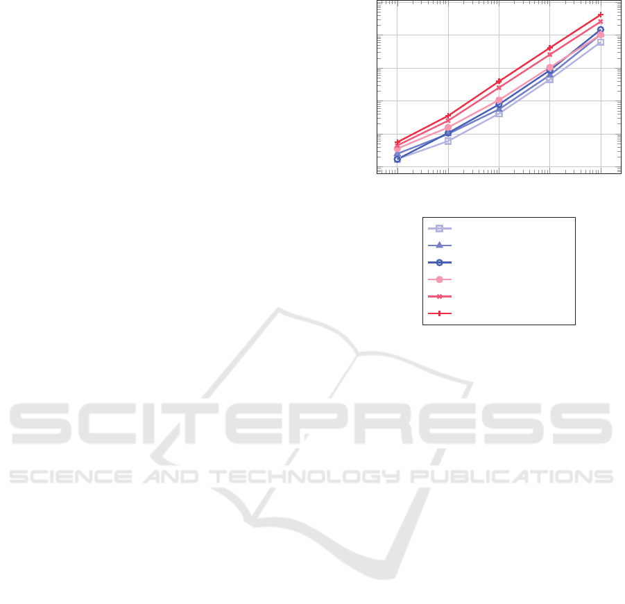
Figure 1: Comparison of execution times for GraphVault

and ArangoDB with different iteration counts.

in higher memory consumption compared to similar

graph databases.

Since ArangoDB currently does not allow indexes

on numeric values within lists, no in-memory indexes

are set on the time intervals in either system. The

graphs are then generated and inserted 10, 30 and

50 times, respectively. After persisting the tempo-

ral graphs in both systems, all historical graphs are

queried over all temporal iterations and the average

query time is calculated. The mean query times of the

comparison are shown in Figure 1 and Table 3.

Our benchmark results demonstrate that Graph-

Vault yields a signiﬁcantly faster query speed (40%-

60%) for graphs as compared to ArangoDB. Graph-

Vault’s efﬁcient ordering of the interval record no-

tably enhances query performance, particularly for

larger graphs. However, our comparison also reveals

that GraphVault’s query speed diminishes with an in-

creasing number of iterations. This is because the vast

number of possible edge combinations results in an

increased generation of new edges, associated prop-

erties and property values with each graph iteration.

These new values must be considered when conduct-

ing a temporal query.

To verify this assumption, a second experiment is

conducted using GraphVault and ArangoDB with 10

nodes and 3 × 10

edges, and a 30% removal proba-

bility. However, the graph is generated only once be-

fore the experiment, and graph elements are dropped

with the given probability per iteration before inser-

ICEIS 2024 - 26th International Conference on Enterprise Information Systems

230

Table 3: Mean execution times for GraphVault and ArangoDB with constantly new values.

Nodes Edges

GraphVault

10 iter. (ms)

ArangoDB

10 iter. (ms)

GraphVault

30 iter. (ms)

ArangoDB

30 iter. (ms)

GraphVault

50 iter. (ms)

ArangoDB

50 iter. (ms)

3 × 10

1.70 3.53 2.47 4.40 1.68 5.543

3 × 10

6.00 15.57 9.87 25.00 10.56 35.102

3 × 10

41.10 105.723 55.47 251.90 77.80 389.754

3 × 10

447.20 1035.00 604.73 2545.00 848.60 4089.00

3 × 10

6111.30 10255.00 10423.27 25698.00 14646.28 41401.00

Table 4: Execution times for GraphVault and ArangoDB

without new values consistently getting 10

nodes and 3 ×

edges inserted.

Iterations GraphVault (ms) ArangoDB (ms)

10 3294.60 8139.00

30 3160.80 10622.00

50 3329.64 13114.00

tion. Therefore, the graph is constantly changing, but

all its components are eventually identiﬁed and can be

reused in GraphVault. The average query times shown

in Table 4 conﬁrm that GraphVault requires a constant

and consistent query time to restructure the graph over

multiple iterations, the increased query times in Ta-

ble 3 are therefore due to the growth of graph data

through time.

5 CONCLUSION AND FURTHER

WORK

Graphs are an excellent data structure for managing

and analyzing a wide variety of data. In this paper

we introduced GraphVault, a graph persistence en-

gine that is capable of storing graph evolutions over

time. We presented our extended labeled property

graph data structure and explained our approach in

mapping it to the key-value engine LMDB through

a speciﬁc record design. Then we concluded by com-

paring the query speed over time between GraphVault

and ArangoDB.

The next step in advancing GraphVault is the im-

plementation of a query engine. The record design is

deﬁned with ﬂexible queries in mind and as such, we

plan to extend a common graph query language with

temporal features and integrate it on top of Graph-

Vault. The objective is to provide high performance

query results that will allow us to effectively ana-

lyze graphs over time in the future. We will evaluate

this feature on both generated and real-world datasets,

demonstrating the potential of temporal graph analy-

sis in practical applications.

REFERENCES

Angles, R., Arenas, M., Barcel

o, P., Hogan, A., Reutter, J.,

and Vrgo

c, D. (2017). Foundations of modern query

languages for graph databases. ACM Comput. Surv.,

50(5).

Belgundi, R., Kulkarni, Y., and Jagdale, B. (2023). Analy-

sis of Native Multi-model Database Using ArangoDB,

pages 923–935.

Campos, A., Mozzino, J., and Vaisman, A. (2016). Towards

temporal graph databases.

Debrouvier, A., Perazzo, M., Parodi, E., Soliani, V., and

Vaisman, A. (2021). A model and query language for

temporal graph databases. The VLDB Journal, 30.

Howard, C. (2015). MDB: A Memory-Mapped Database

and Backend for OpenLDAP.

Kulkarni, K. and Michels, J.-E. (2012). Temporal features

in sql:2011. SIGMOD Rec., 41(3):34–43.

Massri, M., Miklos, Z., Raipin Parvedy, P., and Meye, P.

(2023). Clock-G: Temporal Graph Management Sys-

tem, pages 1–40.

Massri, M., Raipin Parvedy, P., and Meye, P. (2020).

Gdbalive: a temporal graph database built on top of

a columnar data store. Journal of Advances in Infor-

mation Technology, 12.

Miao, Y., Han, W., Li, K., Wu, M., Yang, F., Zhou, L., Prab-

hakaran, V., Chen, E., and Chen, W. (2015). Immortal-

graph: A system for storage and analysis of temporal

graphs. ACM Trans. Storage, 11(3).

NationalSecurityAgency (2016). Lemongraph: Log-based

transactional graph engine — github.com. [Accessed

20-10-2023].

Rita, S. (2021). Graph as The Foundation For Data, Ana-

lytics and AI. Graph + AI Summit, October 5, 2021.

Rost, C., Thor, A., and Rahm, E. (2019). Temporal graph

analysis using gradoop. In Meyer, H., Ritter, N.,

Thor, A., Nicklas, D., Heuer, A., and Klettke, M.,

editors, BTW 2019 – Workshopband, pages 109–118.

Gesellschaft f

ur Informatik, Bonn.

Sadowski, G. and Rathle, P. (2014). Fraud detection: Dis-

covering connections with graph databases. White

Paper-Neo Technology-Graphs are Everywhere, 13.

Salzberg, B. and Tsotras, V. J. (1999). Comparison of ac-

cess methods for time-evolving data. ACM Computing

Surveys, 31(2):158–221.

Vijitbenjaronk, W., Lee, J., Suzumura, T., and Tanase, G.

(2017). Scalable time-versioning support for property

graph databases. pages 1580–1589.

GraphVault: A Temporal Graph Persistence Engine

231