Reinforcement Learning and Optimal Control: A Hybrid Collision
Avoidance Approach
Simon Gottschalk
1 a
, Matthias Gerdts
1 b
and Mattia Piccinini
2 c
1
Institute for Applied Mathematics and Scientific Computing, Department of Aerospace Engineering,
Universit
¨
at der Bundeswehr M
¨
unchen, Werner-Heisenberg-Weg 39, D-85577 Neubiberg, Germany
2
Department of Industrial Engineering, University of Trento, via Calepina 14, 38123 Trento, Italy
Keywords:
Reinforcement Learning, Optimal Control, Collision Avoidance.
Abstract:
In this manuscript, we consider obstacle avoidance tasks in trajectory planning and control. The challenges
of these tasks lie in the nonconvex pure state constraints that make optimal control problems (OCPs) difficult
to solve. Reinforcement Learning (RL) provides a simpler approach to dealing with obstacle constraints,
because a feedback function only needs to be established. Nevertheless, it turns out that often we get a long
lasting training phase and we need a large amount of data to obtain appropriate solutions. One reason is
that RL, in general, does not take into account a model of the underlying dynamics. Instead, this technique
relies solely on information from the data. To address these drawbacks, we establish a hybrid and hierarchical
method in this manuscript. While classical optimal control techniques handle system dynamics, RL focuses
on collision avoidance. The final trained controller is able to control the dynamical system in real time. Even
if the complexity of a dynamical system is too high for fast computations or if the training phase needs to be
accelerated, we show a remedy by introducing a surrogate model. Finally, the overall approach is applied to
steer a car on a racing track performing dynamic overtaking maneuvers with other moving cars.
1 INTRODUCTION
The classical way to approach optimal control tasks is
based on the formulation of the equations of motion,
the definition of an objective function and the repre-
sentation of (e.g. physical) restrictions by constraints.
The resulting optimization problem can then be tack-
led by suitable solvers. It is certainly debatable, when
to define the hour of birth of optimal control theory.
The authors of (Sussmann and Willems, 1997), for
instance, date its birth 327 years ago. However, it is
clear that the solution strategies have been improved
and further developed for a long time. Nevertheless,
since the early 1980s, the development of RL con-
cepts (Sutton and Barto, 2018) is gathering speed.
Nowadays, many new methods enrich the landscape
of approaches which are used to solve control tasks.
It turns out that the data driven way in order to solve
these tasks enables new opportunities. The source
of information in order to find a solution does no
longer need to be given by the designer (e.g. detailed
a
https://orcid.org/0000-0003-4305-5290
b
https://orcid.org/0000-0001-8674-5764
c
https://orcid.org/0000-0003-0457-8777
model, constraints in order to describe the environ-
ment). Now, the information is provided in terms of
data. This leads to a straightforward handling of prob-
lems and to an important link to real world systems,
since a real world system (e.g. a robot) does not need
to be described by an incomplete digital copy. Fur-
thermore, control tasks with high dimensional state
constraints, like constraints for collision avoidance,
can be treated with RL (see e.g. (Feng et al., 2021)).
These constraints make classical OCPs often infea-
sible or hard to solve. Even the dynamic program-
ming methods (Bellman, 1957), which are frequently
used as solver, are reaching their limits. Other au-
thors, like (Liniger et al., 2015; Wischnewski et al.,
2023), try to address this issue by using model predic-
tive control (MPC) in obstacle-free corridors, which
were provided by a higher-level planner. In this way,
nonconvex obstacle constraints can be avoided in the
MPC formulation, but most of the planning effort is
shifted to a higher-level planner.
Nevertheless, RL methods come with problems as
well. Knowledge about the dynamical system, which
might be described well enough by a simple model,
need to be tediously extracted from data. Even the
76
Gottschalk, S., Gerdts, M. and Piccinini, M.
Reinforcement Learning and Optimal Control: A Hybrid Collision Avoidance Approach.
DOI: 10.5220/0012569800003702
Paper published under CC license (CC BY-NC-ND 4.0)
In Proceedings of the 10th International Conference on Vehicle Technology and Intelligent Transport Systems (VEHITS 2024), pages 76-87
ISBN: 978-989-758-703-0; ISSN: 2184-495X
Proceedings Copyright © 2024 by SCITEPRESS – Science and Technology Publications, Lda.

simplest information needs to be learned first.
In the last decade, many approaches have been es-
tablished trying to prevent RL from inefficient learn-
ing. For instance, besides the model free RL methods,
model based methods are investigated as well. In the
model based version of RL, the RL idea is extended
by a model of the system dynamics. The dynamics
are either learned from data itself or a model is al-
ready known at the beginning. For an overview of
model based RL approaches, we recommend the sur-
vey (Moerland et al., 2020). Another idea to simplify
the training procedure is Hierarchical Reinforcement
Learning (HRL). Here a complex task is divided into
subtasks and multiple RL agents act on different lev-
els of details. We refer to (Pateria et al., 2021) for
a deeper insight into the working principle of HRL
and methods based thereon. Furthermore, there is
the class Imitation Learning (IL) (Attia and Dayan,
2018), where an expert’s action is imitated (respec-
tively learned). The learned behavior is then applied
to sequential tasks.
We stress at this point that the information source
for model based RL, HRL and IL is still mainly en-
coded in data. Ideas, which include classical planning
or optimal control techniques and thus a different in-
formation source are given in a hybrid method (Reid
and Ryan, 2000) and in the method of the authors
of (Landgraf et al., 2022). The former one decides
to use, similar to the method we will present in this
manuscript, two stages. On a coarse grid, a planning
algorithm is used, while on a finer grid, RL is used.
The latter one combines a RL agent with a MPC unit.
The idea is that the RL algorithm is used to decide if
an obstacle (e.g. on a street) is overtaken on the left or
the right hand side. Then the MPC unit actually steers
the vehicle in a collision free manner.
In the field of physics-informed Reinforcement
Learning (PIRL), physical knowledge is incorporated
into RL approaches in order to increase the efficiency
of the training. A survey could be found in (Banerjee
et al., 2023). For instance, physical knowledge could
be used in a model-based RL framework (Ramesh and
Ravindran, 2023), where it is used to find a suitable
approximation model. We are interested in benefiting
from a hierarchical and knowledge-based framework,
which leads us to our approach in this manuscript.
In this manuscript, we will introduce a hierarchi-
cal method, which uses the strengths of RL and classi-
cal approaches for OCPs on different stages. We will
use RL in order to plan a geometric path on a coarse
grid and consider an OCP on a finer grid. Thereby,
our approach differs from the above addressed hy-
brid method, where RL was used on the finer grid.
The hierarchical structure resembles more the struc-
ture in (Landgraf et al., 2022). However, we are con-
vinced that we can benefit even more from RL and
OCP, if we combine them differently. Instead of let-
ting the RL method manipulate the objective function
of a MPC problem in order to push the car to the left
or the right, we let RL influence the constraints of an
OCP by setting initial and target positions. In other
words, this means that we separate the overall task
into a collision avoidance task and a steering task of
the actual dynamical system. The RL part finds suit-
able waypoints for a subsequent trajectory optimiza-
tion. Between those waypoints the classical optimal
control approach solves a start to end control problem
without any collision avoidance constraint. The con-
nections between these parts are on the one hand that
RL defines the initial and target position of the OCP
and that the optimized trajectory is led back to the up-
per level such that collision avoidance is again take
care of by RL. Furthermore, since the OCP needs to
be solved many times during training and the final ap-
plication, we introduce a strategy in order to quickly
get a good solution approximation of the OCP.
This manuscript is structured as follows: We be-
gin with a detailed description of the working princi-
ple of the novel approach in Section 2. Therein, we
introduce the OCP principle in Subsection 2.2 as well
as the basics of RL in Subsection 2.1. In Subsection
2.3 we focus on the algorithm itself. The surrogate
model in order to reduce the duration of the RL train-
ing phase is introduced in Subsection 2.4. In Section
3, we apply the previously described approach to an
autonomous path planning scenario.
2 HYBRID METHOD
Let us start with the classical setup of optimal control
problems for collision avoidance tasks. The goal is
to compute a collision free trajectory of a dynamical
system from an initial state x
init
to a target state x
end
on the time interval [t
0
,t
f
]. The outcome of the opti-
mization problem is a trajectory x(t) from the space
of absolutely continuous functions W
1,∞
([t
0
,t
f
], R
n
x
)
and a control u(t) from the space of essentially
bounded functions L
∞
([t
0
,t
f
], R
n
u
) (see (Gottschalk,
2021, pp.22 ff.)), which will be abbreviated by W
1,∞
and L
∞
from now on. Here n
x
∈ N
>0
and n
u
∈ N
>0
de-
note the dimensions of the state and the control vec-
tors. The objective function is defined by the func-
tions ϕ : R
n
x
× R
n
x
→ R and f
0
: R
n
x
× R
n
u
→ R. The
former one contains the goals for the initial and end
states, while the latter one is integrated over the whole
time interval. The dynamical system is given by
equations of motion. The ordinary differential equa-
Reinforcement Learning and Optimal Control: A Hybrid Collision Avoidance Approach
77

tion of order one is defined by the right hand side
f : R
n
x
× R
n
u
→ R
n
x
. The initial and final state can
be either specified by additional initial and final con-
straints or by the objective function ϕ. Furthermore,
pure state constraints g
st
: R
n
x
→ R
n
gx
with n
gx
∈ N
for the collision avoidance appear in the optimization
problem. Overall, the problem can be stated as (see
also (Gerdts, 2024)):
min
x∈W
1,∞
u∈L
∞
ϕ(x(t
0
), x(t
f
)) +
Z
t
f
t
0
f
0
(x(t), u(t))dt (1a)
s.t. ˙x(t) = f (x(t), u(t)), (1b)
x(t
0
) = x
init
, x(t
f
) = x
end
, (1c)
g
st
(x(t)) ≤ 0. (1d)
Now, the idea of this manuscript is that the pure
state constraints (1d) are separated from the optimiza-
tion problem, since they make the problem hard to
solve. Therefore, we partition the whole problem into
smaller sub-problems, which are concatenated by the
RL approach. The RL part includes the pure state con-
straints and generates a collision free geometric path
on a coarse grid, while an OCP without pure state con-
straints computes the actual trajectory.
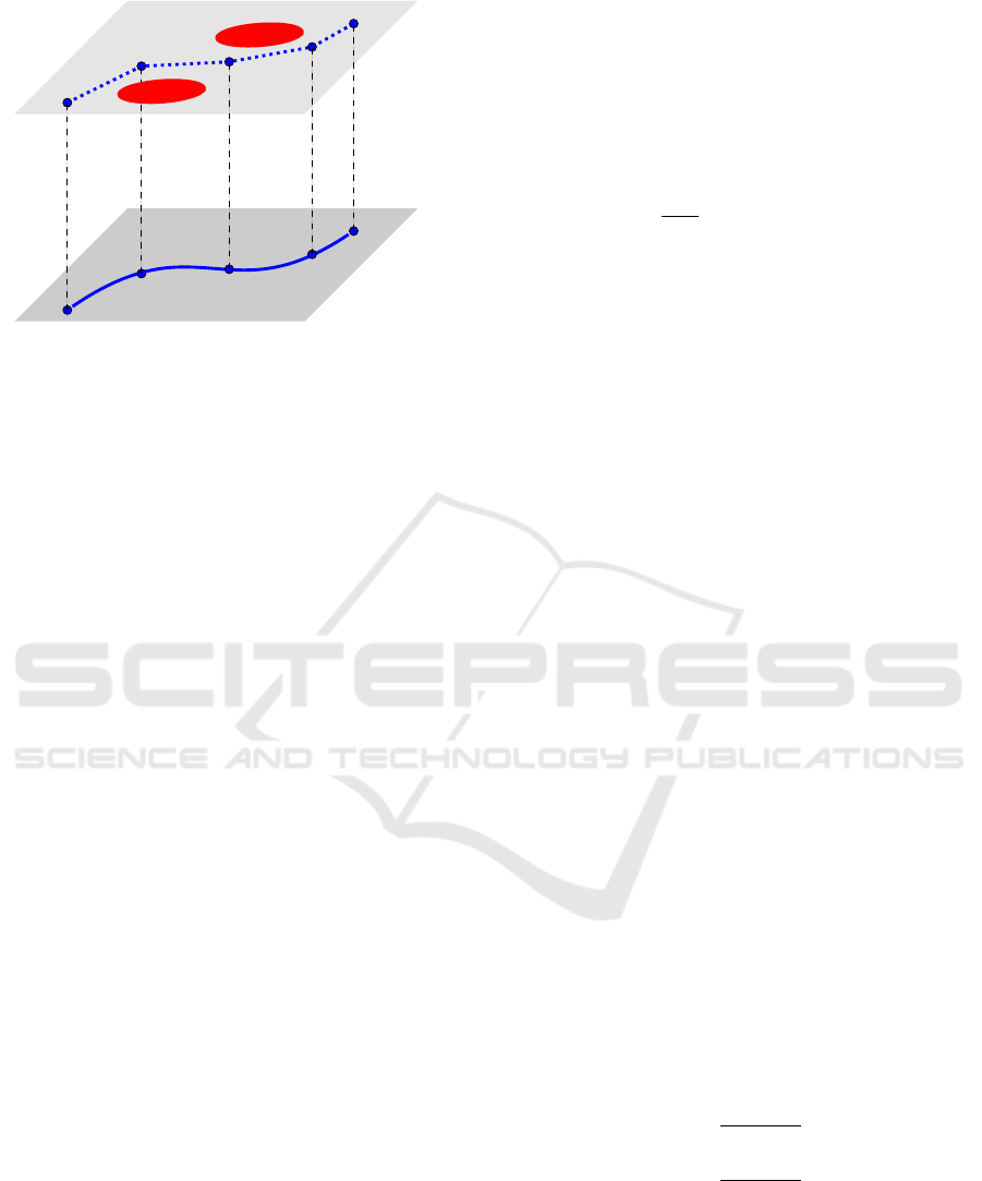
In the following, we sketch the structure of the
method in Figure 1. For illustrative purposes, we
choose a two dimensional collision avoidance prob-
lem and refer to it in our explanations. Thus, for ex-
ample, we can think of a car, which tries to avoid the
red obstacles. Now, we split the problem into two
sub-problems. The obstacle avoidance stays in the
RL stage, while the optimal trajectory of the dynami-
cal system (model of the car) is solved by a classical
OCP solver. Overall, RL sets the next waypoint s
k+1
and then an OCP is solved to actually steer the car
from the current waypoint x
init
= s
k
to the next one
x
end
= s
k+1
. The trajectory x
k
(t), which we get from
the OCP, where no collision constraints appear, is then
checked for collisions and a feedback goes to the RL
routine. In this way, we use the RL approach for the
creative part, where we need to find a valid route and
the OCP for handling the dynamics, which we de-
scribe by an analytical model. Based on the feedback
from the trajectory, the RL algorithm can iteratively
improve the waypoints.
The main components for this approach, namely
the RL and OCP problem, are introduced in the fol-
lowing.
2.1 Reinforcement Learning
On the upper stage of Figure 1 we have RL (Sut-
ton and Barto, 2018) for the computation of a col-
lision free geometric path. The underling struc-
ture is a feedback control loop. Based on the cur-
rent state (waypoint of the geometric path) an ac-
tion is generated in order to get the next state based
on the old state and the action. Mathematically,
RL’s basis is a Markov Decision Process (MDP)
(Feinberg and Shwartz, 2002), which consists of a
state space S, an action space A, a transition dis-
tribution P : S × A × S → [0, 1], an initial distribution
P
0
: S → [0, 1] and a reward function r : S × A → R.
The state, respectively action space, are the sets of
all possible states, respectively actions. The transi-
tion distribution P represents the underlying dynam-
ical system. Instead of assuming to have equations
of motion, we content ourselves with the knowledge
of the probabilities of the next state, when the current
state and action are known. Thereby, the very first
state is described by the initial distribution. Finally,
the reward function gives us feedback about the cur-
rent control strategy. The missing part of the control
loop is the controller itself. It is the overarching goal
to find this controller. More precisely, we are inter-
ested in a transition distribution - in this context called
policy - π : A × S → [0, 1], which leads to actions with
the best reward. We denote a trajectory by listing the
corresponding states and actions, i.e.
τ = [s
0
, a
0
, . . . , a
n−1
, s
n
], for s
k
∈ S, a
k
∈ A, ∀k, (2)
We denote the space of all possible trajectories
Γ := S × A × ··· × S. The corresponding optimization
problem can be stated as follows:
max
π
E
τ
[R(τ)] :=
∑
τ∈Γ
¯
P(τ|π)R(τ), (3a)
with R(τ) :=
n−1
∑
k=0
γ
k
r(s
k
, a
k
) and (3b)
¯
P(τ|π) := P
0
(s
0
)
n−1
∑
k=0
P(s
k+1
|a
k
, s
k
)π(a
k
|s
k
), (3c)
where 0 < γ ≤ 1 is a discount factor to discount fu-
ture rewards. Note that the above notation is based
on the assumption that the state and action space are
finite. This was done to provide a better overview and
is no restriction. For an infinite formulation, one can
follow the notation of (Gottschalk, 2021). Several
types of RL approaches are known in order to solve
optimization problem (3a) (e.g.Value Iteration and Q-
Learning (Bertsekas, 2019), REINFORCE (Williams,
1992), DPG (Silver et al., 2014), TRPO (Schulman
et al., 2015)). For our application in this manuscript,
we make use of the straightforward Value Iteration
(VIter). Nevertheless, we stress that all other ap-
proaches can be easily integrated in the described hy-
brid approach.
In case of VIter, the policy is not trained directly,
but a value function V : S → R is built up successively.
VEHITS 2024 - 10th International Conference on Vehicle Technology and Intelligent Transport Systems
78

RL
OCP
s
0
s
1
s
2
s
3
s
4
x
0
(t)
x
1
(t)
x
2
(t)
x
3
(t)
Figure 1: Sketch of the idea of the hybrid approach.
The update formula, which is motivated by Bellman’s
equation (see (Bellman, 1957)), reads for s ∈ S:
V
k+1
(s) = max
a∈A
r(s, a) + γ
∑
s
′
∈S
P(s
′
|s, a)V
k
(s
′
). (4)
After the sequence has converged to V , the value func-
tion implicitly provides a policy:
a := argmax
a
′
∈A
r(s, a
′
) + γ
∑
s
′
∈S
P(s
′
|s, a
′
)V (s
′
) (5)
Therefore, every time we have to make a decision, we
choose the action, which leads to the largest value.
Finally, the collision avoidance needs to be inte-
grated in the reward function. We can only rate the
waypoints by having a feedback, whether there is a
collision in between those waypoints or not. The
computation of the actual trajectory in between of
these waypoints is provided by the OCP part, which
is introduced in Subsection 2.2.
2.2 Optimal Control with ODEs
In this subsection, we focus on the OCP part. It was
introduced to steer the dynamical system from a given
initial position s
k
to a target position s
k+1
on the time
interval [t
0
,t
f
]. The mathematical formulation of this
parametric OCP (s
k
, s
k+1
) can be written as:
min
x∈W
1,∞
u∈L
∞
ϕ(x(t
0
), x(t
f
)) +
Z
t
f
t
0
f
0
(x(t), u(t))dt (6a)
s.t. ˙x(t) = f (x(t), u(t)), (6b)
x(t
0
) = s
k
, x(t
f
) = s
k+1
. (6c)
Problem (6) differs from problem (1) in the con-
straints, where we do not have the pure state con-
straints for the collision avoidance. We ensure to
have a unique solution of the ordinary differential
equation by assuming that the function f satisfies
a global Lipschitz-property. Then, the theorem of
Picard-Lindel
¨
of (e.g. (Gr
¨
une and Junge, 2008)) leads
to the desired existence.
To solve the OCP (6), we proceed by discretizing
it. We use the explicit Euler rule even if there are
many other possibilities, which would leave the fol-
lowing steps unaffected. The discretized optimization
problem for an equidistant discretization of the time
interval t
0
,t
1
, . . . , t
N
= t
f
for N ∈ N with equidistant
time steps (h :=
t
f
−t
0
N
) has the form:
min
x
i
,u
i
ϕ(x
0
, x
N
) +
N−1
∑
i=1
h f
0
(x
i
, u
i
) (7a)
s.t. 0 = x
i+1
− x
i
− h f (x
i
, u
i
),
∀i ∈ {0, . . . , N − 1}
(7b)
0 = x
0
− s
k
, (7c)
0 = x
N
− s
k+1
. (7d)
In the remainder of this subsection, we aim to refor-
mulate problem (7) into a system of equations. The
reason is that we will use it to define the objective
function in Subsection 2.4 in order to train a neural
network, which outputs the solution of the OCP with
respect to the initial and target position directly.
Thus, we consider the KKT conditions (Karush,
1939)(Kuhn and Tucker, 1951) of problem (7). We
mathematically introduce them via the corresponding
Lagrange function, which is given by
L (X, Λ) = ϕ(x
0
, x
N
) +
N−1
∑
i=1
h f
0
(x
i
, u
i
) + λ
T
N
(x
0
− s
k
)
+
N−1
∑
i=0
λ
T
i
(x
i+1
− x
i
− h f (x
i
, u
i
)) + λ
T
N+1
(x
N
− s
k+1
),
(8)
where X and Λ are defined as follows:
X =

x
T
0
, x
T
1
, . . . , x
T
N
, u
T
0
, u
T
1
, . . . , u
T
N

T
and (9)
Λ =

λ
T
0
, λ
T
1
, . . . , λ
T
N+1

T
. (10)
Based on (8), the KKT conditions for (7) can be de-
rived. The derivatives of the Lagrange function with
respect to X, as well as Λ yield the KKT conditions:
0 =
∂L (X, Λ)
∂X
, (11a)
0 =
∂L (X, Λ)
∂Λ
. (11b)
Remark. Note that the OCP (6) might have con-
straints for the control in the form of g
con
(u(t)) ≤ 0
with g
con
: R
n
u
→ R
n
gu
, n
gu
∈ N. We mentioned that
pure state constraints (for collision avoidance) can
be outsourced to RL, but possible restrictions for the
control might appear anyway. In the case of inequality
Reinforcement Learning and Optimal Control: A Hybrid Collision Avoidance Approach
79

control constraints in the KKT conditions, those can
be transformed into non-smooth equality equations
by the Fischer-Burmeister function (Fischer, 1992).
Additional control constraints do not weaken this ap-
proach since the important part is that high dimen-
sional pure state constraints are handled by RL.
For a better overview, we simplify the system of
equations by introducing a new function, which rep-
resents the KKT conditions from (11):
G(X, Λ, s
k
, s
k+1
) = 0. (12)
For instance, (12) could be solved by a New-
ton method (Deuflhard, 2011) or, in the case of
non-smooth equations, by the semi-smooth Newton
method (Ito and Kunisch, 2009). Then, the over-
all solution strategy would be the Lagrange-Newton
method (Gerdts, 2024, pp.228 ff.). Nevertheless, in
this manuscript, we will train a neural network to
these KKT conditions (see Subsection 2.4). This pays
off since problem (6) has to be solved many times and
hence, the overall approach requires a quick solution
method. We now describe the overall structure of the
hybrid approach.
2.3 The Overall Approach
The overall flow chart of the described approach can
be seen in Figure 2. In an outer loop the RL algo-
rithm generates waypoints, which are visited one af-
ter the other. Thereby, the actual control in order to
steer the system (e.g. the car) comes from the OCP.
Furthermore, the result of the OCP is also used in or-
der to compute the reward for the value function up-
date during the training phase of the RL algorithm.
We have seen in (3a) that the rewards form the objec-
tive function during the training. The reward function
needs to be tailored to the application case. From a
collision avoidance point of view, it is clear that this
function penalizes collisions along the computed tra-
jectory with obstacles. Beyond that, we can define,
for instance, the rewards such that they are influenced
by the OCP objective function (6a). Other terms can
consist of penalties for the control effort or minimum
time terms.
After the training, the implicit policy, which only
has to evaluate the value function, can make very fast
decisions, where to go next. And since we constructed
the OCP in a simple way, we expect that the overall
procedure provides a sufficiently fast controller. Of
course, this highly depends on the dynamical system
itself and the question of how quickly decisions have
to be made. Nevertheless, in the RL training algo-
rithm, we need to solve many OCP problems in or-
der to compute the rewards. Thus, the time needed to
a
k
s
k+1
u
P(s
k+1
|a
k
, s
k
)
a
k+1
= arg max
a
′
∈A
r(s
k+1
, a
′
) + γ
∑
s
′
∈S
P(s
′
|s
k+1
, a
′
)V (s
′
)
min
x,u
ϕ(x(t
0
), x(t
f
)) +
Z
t
f
t
0
f
0
(x(t),u(t)) dt
s.t. ˙x(t) = f (x(t), u(t)),
x(t
0
) = s
k
, x(t
f
) = s
k+1
.
r
k
V
Figure 2: Flow chart of the hierarchical method.
solve the OCP (6) highly influences not only the final
procedure, but also the training period. We will now
present a way in order to accelerate the OCP part.
2.4 Surrogate Model for the Optimal
Control Problem
Note again that the runtime of a solver for problem (6)
highly depends on the complexity of the right hand
side function f of the ordinary differential equation.
Since the solution is necessary for the final control
approach as well as its training routine, the computa-
tional time of the solver is crucial.
Introducing surrogate models for the OCP is a
possibility to decrease the training time of the RL ap-
proach. Several different surrogate models are possi-
ble. For instance:
• The function f could be replaced by a simplified
model described by
˜
f . The OCP (6) for the re-
placed equations of motion would be simplified
and would lead to cheaper computations of the re-
wards. Nevertheless, for the final controller, we
would need the original right hand side function
in order to compute the correct controls of the dy-
namical system.
• Splines (de Boor, 1978) could be used to approx-
imate a trajectory between the initial and target
point. During the training this could be used to
solve coarse collision avoidance tasks, where a
safety distance for deviations is included into a
buffer. Obviously, this surrogate model can only
be used in the training phase, since in the final
controller the actual controls need to be com-
puted.
We prefer another possibility, which is based on
machine learning. We remember that, in order to re-
place the OCP (6), we need to find a model, which
maps the way points s
k
and s
k+1
to the trajectory and
the corresponding controls. Thus, we are interested
VEHITS 2024 - 10th International Conference on Vehicle Technology and Intelligent Transport Systems
80

in a parametric approximator h
θ
with parameters θ,
which we train by generated data. The approxima-
tor can have different forms. For instance, neural
networks and radial basis functions are well suited.
Such an approximator can be trained by supervised
learning or a knowledge-informed method based on
(De Marchi et al., 2022), which we will use in this
manuscript. Let us start with the classical supervised
approach in order to motivate our approach.
In the classical supervised learning framework,
we solve the OCP (6) for representative initial and
end states. These solutions are stored and used
for the training. The overall training data then
would consist of the initial and end states as in-
put data and the solution trajectory and control as
output data. Let us denote the training pairs with

S
l
=

s
l
, ˜s
l

, X
l

l=1,...,L
, L ∈ N. Here, s
l
represents
the initial state and ˜s
l
the target state of the OCP (6).
The output of the training data X
l
contains the union
of states and controls as well as the multipliers, if de-
sired, of the KKT points. Then, our goal is to find a
parameterized mapping h
θ
with h
θ
(s
l
, ˜s
l
) = X
l
. In or-
der to train the parameters with supervised learning,
the following optimization problem is solved:
min
θ
1
2
L
∑
i=1
∥h
θ
(s
l
, ˜s
l
) − X
l
∥
2
. (13)
In order to solve such a problem, a gradient, a Gauss-
Newton or the Levenberg-Marquardt method are suit-
able approaches. In the case of a neural network
approximator, the efficient backpropagation approach
(Rumelhart et al., 1986) is another alternative. The
disadvantage of this approach lies in its black-box
manner. It is not clear whether the trained solution
generalizes from the training set to unseen scenarios.
Thus, we apply a knowledge-informed approach
based on (De Marchi et al., 2022). It is based on the
idea to interpret the OCP (7) as a parametric optimiza-
tion problem with parameters [s
T
k
, s
T
k+1
]. Following
the idea of (De Marchi et al., 2022), the goal is to find
a parametric solution approximator (h
θ
(s
k
, s
k+1
)) of
the corresponding solution X(s
k
, s
k+1
) with adjustable
values θ. We decided to use the same notation for the
approximator as for the parameterized mapping in the
supervised learning. The reason is that they are struc-
turally the same and address the same tasks. Only the
method for the training differs. Here, the KKT con-
ditions (12) from Subsection 2.2 can be transformed
into the nonlinear least squares problem for training
waypoints (s
l
, ˜s
l
)
l=1...,L
, L ∈ N:
min
θ,Λ
ˆ
J(θ, Λ) :=
L
∑
l=1
∥G(h
θ
(s
l
, ˜s
l
), Λ, s
l
, ˜s
l
)∥
2
. (14)
In other words, the parameters θ of the solution ap-
proximator are trained by minimizing the residuals
of the KKT conditions. We emphasize that the au-
thors of (De Marchi et al., 2022) introduce a theoreti-
cal error estimation for this approach, which consists
mainly of the norm of the KKT conditions.
The great advantage of this machine learning ap-
proach is that the approximator can not only be used
in the training phase, but also in the real application.
In such a way the computing time can be reduced
rapidly, since only neural networks (or other approxi-
mators) need to be evaluated. In our numeric section
we show that for our application the computing time
is reduced by more than twenty times.
Now, we have everything at hand in order to apply
the above hybrid approach to our application case.
3 NUMERICAL RESULTS
In this section, we introduce a dynamic vehicle model
on a roadway described by clothoids. The main task is
to avoid collisions with other road users, which move
along the road and change lanes randomly. Based on
this example, we will illustrate all the above described
steps.
First, we focus on the model in order to steer a
car on a given track. There are many different mod-
els in the literature, which describe the behavior of a
car on different detail levels. We use a kinematic ve-
hicle model in accordance with the models described
in (Pagot et al., 2020) and (Lot and Biral, 2014). We
assume that the center-line of the road is given by a
curvature, which is only changing linearly on a given
horizon. Thus, we assume that on a track section the
curvature is given as κ = k
1
+ k
2
ζ. Thereby, ζ is the
curvilinear abscissa of the road center-line. k
1
and
k
2
are given parameters of the track. Given this as-
sumption, the car is represented by four variables x
s
,
x
n
, x
α
and x
Ω
. x
s
describes the curvilinear abscissa
of the path traveled by the car and x
n
the lateral de-
viation from the center-line. The angle x
α
denotes
the relative yaw angle of the vehicle with respect to
the road center-line and x
Ω
the yaw rate of the vehi-
cle. For the sake of simplicity, the velocity v = 5
m
s
of the car is fixed. Please note that the equations of
motion can be easily extended to model variable vehi-
cle velocity and longitudinal acceleration (see (Pagot
et al., 2020)). The overall model on a road section
Reinforcement Learning and Optimal Control: A Hybrid Collision Avoidance Approach
81

ζ ∈ [0, L
H
] has the form:
dx
s
(ζ)
dζ
=1 − x
n
(ζ)(k
1
+ k
2
ζ), (15)
dx
n
(ζ)
dζ
=x
α
(ζ), (16)
dx
α
(ζ)
dζ
=
x
Ω
(ζ) − (k
1
+ k
2
ζ)v
v
, (17)
dx
Ω
(ζ)
dζ
=
u(ζ)
v
. (18)
In the example below, we use L
H
= 20m. Further-
more, the control u is the yaw acceleration of the ve-
hicle. Note that the derivatives here are with respect
to the arc length and not the time. Nevertheless, this
only entails that the arc length replaces the time in the
optimization problem (6). For the dimension of the
car, we choose the width 2m and the length 3m. That
is about the size of a compact car. The differential
equations represent equation (6b) in our original op-
timization problem. Additionally, we need to define
our goals in terms of the objective function. Since
strong steering always leads to high forces which act
on the passengers and make them feel uncomfortable,
we aim to suppress it if it is not absolutely necessary.
Thus, we minimize the control effort, which can be
seen as a maximization of the passengers’ comfort,
by using:
J(x, u) =
Z
L
H
0
u(ζ)
2
dζ. (19)
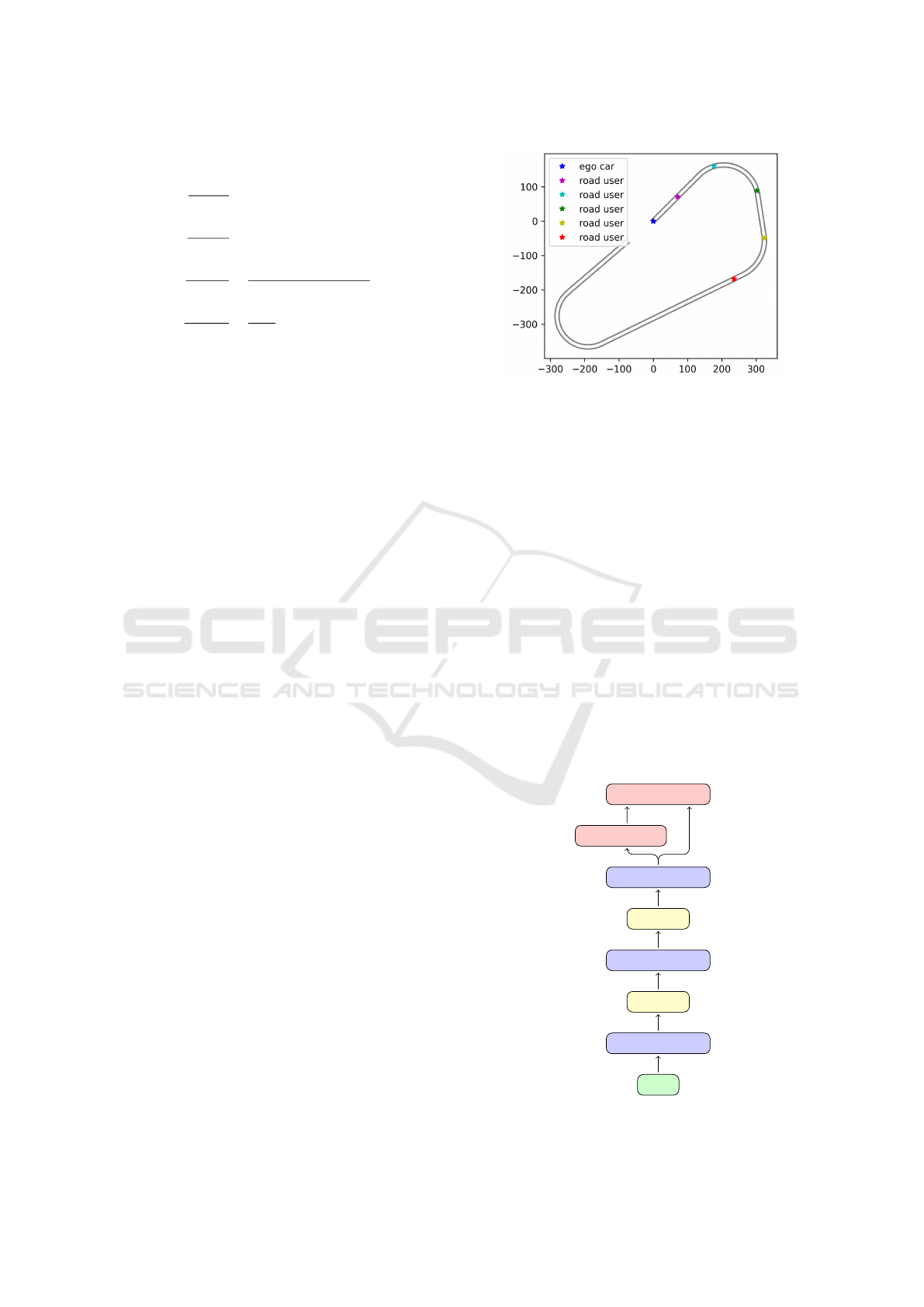
The road, which we would like to follow can be seen
in Figure 3. The stars in the figure represent the start-
ing point of our car (blue) and other road users (col-
orful). These road users are driving on the course
with half of our velocity such that we have to over-
take them. Thereby, these vehicles change road lanes
randomly.
3.1 Neural Network Approximation of
the OCP
At this point, we have the differential equation and
objective function and we can focus on the optimiza-
tion problem 6. The initial state s
k
and end state s
k+1
are considered as parameters of the problem. Follow-
ing Subsection 2.2 and Subsection 2.4, we discretize
the optimization problem and end up with equation
G(X, Λ, s
k
, s
k+1
) = 0. (20)
Our goal is to find the parameterized mapping
h
θ
(s
l
, ˜s
l
) = X
l
, which maps the training parameters to
the actual trajectory and controls. Therefore, we need
to define the training parameters (s
l
, ˜s
l
)
l=1...,L
, L ∈ N
Figure 3: The considered Course and start positions. blue =
vehicle to be steered. colorful = other road users.
and need to specify, which approximator we would
like to use. As the latter, we use a neural network,
which maps the parameters to the controls, and after-
wards equation (7b) is applied to generate the corre-
sponding trajectory. The neural network consists of
three hidden layers, where the first and second one
each contain 64 neurons, which was determined by
a grid search approach. Furthermore, the hyperbolic
tangent is used as activation function. The last layer
consists of 30 neurons and the activation function is
the identity. A sketch of the network can be found in
Figure 4.
Note that the multipliers Λ need to be optimized
as well. But since we do not need the multipliers
for the trajectory approximation, we treat them as free
optimization variables and throw them away after the
training.
For the training parameters, we set up scenar-
ios. In this way, we decide that the car’s orientation
s
l
, ¯s
l
fully connected
64
tanh
64
fully connected
64
tanh
64
fully connected
equation (7b)
30
X
Figure 4: Scheme of the neural network approximation.
VEHITS 2024 - 10th International Conference on Vehicle Technology and Intelligent Transport Systems
82

Iterations
log

ˆ
J(θ, Λ)

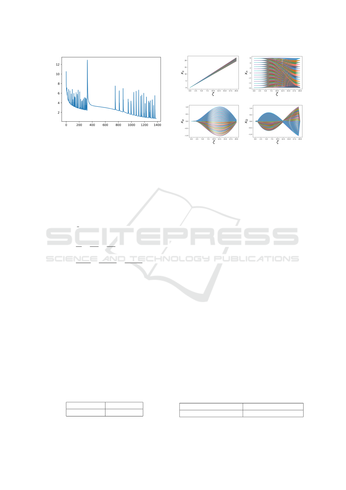
Figure 5: Training progress.
shall direct in the direction of the street at the ini-
tial and target state. Thus, we set for the initial and
final state the orientation variables x
α
and x
Ω
equal
to zero. Note that obviously in between x
α
and x
Ω
can be different from zero. Furthermore, the hori-
zon length in the OCP is set to L
H
= 20m, which
was found to provide satisfactory performance. Fi-
nally, we set x
s
= 0, which is no further restriction
here. So the following parameters remain: initial and
target value for x
n
. For the training data, we allow as
initial and target deviations from the center-line dis-
tances of {±k
5
6
[m]|k = 0, . . . , 7}. For the curvature,
we allow:
k
1
∈

0, ±
1
90
, ±
1
100
, ±
1
110

and (21)
k
2
∈

0, ±
1
90 · 20
, ±
1
100 · 20
, ±
1
110 · 20

. (22)
At this point, we can solve the optimization prob-
lem (14) in order to find the optimal weights of the
neural network. We apply the ADAM optimizer
(Kingma and Ba, 2014) (step size 1e − 2, decaying
every 1000 steps by a factor of 0.9) implemented in
TensorFlow (Abadi et al., 2015).
The training progress can be observed in Figure
5. It shows the logarithm of the objective function
from (14) for each iteration. We observe that the ob-
jective function becomes small, which is what we ex-
pected. We draw the trajectories, which result from
the trained neural network applied to the training data,
in Figure 6. The trajectories look smooth and they
seem to achieve the desired target position in the train-
ing data. The corresponding controls are plotted in
Figure 7.
Table 1: Average error in the target position. Comparison
of the test and training data.
Training Data Test Data
≈ 2.16 · 10
−2
≈ 2.63 · 10
−2
Figure 6: Trajectory for all scenarios after training.
Furthermore, we compare the performance of the
neural network on the training and on 1000 random
test data. The initial and target position for the test
data are drawn uniformly. For the comparison, we
need to understand that it is not possible to evalu-
ate the function G from (20), since the neural net-
work does not provide the multipliers for the test data.
Thus, we use the neural network to compute the con-
trols for the training data as well as for the test data.
For these controls, we generate the trajectories by
solving (7b) and evaluate the deviation between the
computed target position and the desired target posi-
tion. The average errors are listed in Table 1. We
deduce that the training was successful and the neural
network is generalizable to unseen test data.
In Table 2 we list the average computation time,
which is needed to get the trajectory from the trained
neural network. We compare it to the average time,
which a Python optimization solver takes to solve the
discretized optimal control problem (7). We observe
that the neural network generates the trajectory in less
than 1 ms, while the classical optimization takes more
than 20 times longer. We emphasize that the total
training time of the RL approach is significantly re-
duced by the neural network, because of the large
number of trajectory calculations required. We ex-
pect that for more complex dynamical systems, the
difference in computation time becomes even higher.
3.2 Value Iteration
In the RL part, we apply the VIter approach. As de-
fined in Section 2.1 we need to define the MDP of our
Table 2: Average computation times. Comparison of the
classical OCP solver and the trained neural network.
Computation Time OCP Computation Time NN
≈ 14.51 ms ≈ 0.68 ms
Reinforcement Learning and Optimal Control: A Hybrid Collision Avoidance Approach
83

Figure 7: Controls for all scenarios after training.
problem. At first, we focus on the state space S. From
the previous subsection, we know that, in order to get
a trajectory from the neural network, the initial and
target lateral deviation from the center-line has to be
determined. Thus, the state space can be defined as
S := {−5., −2.5, 0., 2.5, 5.} × {m · L
H
|m ∈ N}, (23)
where the first component represents the deviation
from the center-line and the second component indi-
cates the road section, where the car is located.
Obviously, the corresponding actions need to pro-
vide information about the deviation from the center-
line after the next road section. Thus, we define the
action space as
A := {−5., −2.5, 0., 2.5, 5.}. (24)
Based on this, the transition probability can be de-
fined. Given a current state s ∈ S and an action a ∈ A,
the next state would be s
′
:= [a, s
2
+ 20], where s
2
rep-
resents the second component of s. In the case that
we would like to model a given uncertainty in order
to increase the robustness, we can add a probability of
occurrence p = 0.85 and we get
P([a, s
2
+ 20]|s, a) = p and (25)
P([ ˜a, s
2
+ 20]|s, a) =
1 − p
4
, ∀ ˜a ∈ A \ {a}. (26)
Note, that knowing explicitly the transition probabil-
ity is not necessary for all RL approaches, but for
VIter. In case of absence, other techniques could be
used.
It remains to define the reward function for the
MDP. Here, we stick to the most important features
our trajectory should have:
i) A collision with another car should be avoided.
ii) The ego car should not change too many lanes at
the same time if it is not necessary.
iii) We want that the car drives on the inside lane in a
road corner and in the middle of the street every-
where else, if possible.
ˆx
α
ˆx
n
x
α
x
n
Figure 8: Collision avoidance scenarios.
The trajectory segments can be computed with the
trained neural network from the previous section. The
mapping h
θ
(s
k
, s
k+1
) gives us the trajectory from s
k
to
s
k+1
. Thus, for the collision avoidance we consider
the trajectory points x(ζ
0
), . . . , x(ζ
N
) at the equidis-
tant grid points ζ
i
between s
k
and s
k+1
. Additionally,
we take the trajectory ˆx(ζ
0
), . . . , ˆx(ζ
N
) of the other
road user, who is at the same time on the same road
section as we are.
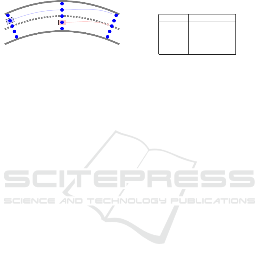
i) Based on this, we check a collision as sketched
in Figure 8. In short, we check, if one of our corners
enters the other vehicle. We compute:
cor
j
:=

ζ
i
x
n

+

cos(x
α
) −sin(x
α
)
sin(x
α
) cos(x
α
)

v
j
, (27)
ˆ
cor
j
:=

ˆ
ζ
i
ˆx
n

+

cos( ˆx
α
) −sin( ˆx
α
)
sin( ˆx
α
) cos( ˆx
α
)

v
j
, (28)
v
1
=

1.5
1

, v
2
=

1.5
−1

, v
3
=

−1.5
1

, v
4
=

−1.5
−1

,
∀ j = 1, . . . , 4 and ζ
i
= 0, . . . , N.
Here, 1m and 1.5m are half of the width, respec-
tively length of the car, and
ˆ
ζ
i
is the curvilinear
abscissa of the other road user at the same time,
when the ego car is at ζ
i
. If one of the corner
points cor
j
lies in the rectangle spanned by the points
ˆ
cor
j
, j = 1, . . . , 4, we detected a collision and the re-
ward becomes r
1
(s
k
, s
k+1
) = −10. Otherwise, it is
zero.
ii) The second part penalizes the number of lane
changes, which we do in the next step:
r
2
(s
k
, s
k+1
) = −0.1
|s
k,1
− s
k+1,1
|
2.5
. (29)
Here s
k,1
and s
k+1,1
denote the first component of s
k
,
respectively s
k+1
. This suppresses strong maneuvers,
if they are not necessary.
iii) The third part of the reward ensures that the
VEHITS 2024 - 10th International Conference on Vehicle Technology and Intelligent Transport Systems
84

ζ = 0m
ζ = 20m
ζ = 40m
Figure 9: Scenarios for the VIter training.
car takes the inner lane in curves, if possible:
r
3
(s
k
, s
k+1
) =
(
−0.175 ·
|s
k+1,1
|
2.5
, if κ = 0
−0.175 ·
(|s
k+1,1
−5·sign(κ))|
5
, else.
(30)
Overall, the reward is defined as:
r(s
k
, s
k+1
) = r
1
(s
k
, s
k+1
) + r
2
(s
k
, s
k+1
) + r
3
(s
k
, s
k+1
).
(31)
Based on this defined MDP, we can now apply the
VIter method. This means, we need to find the value
function V (s
k
). We use a 5
2
× 3 × 100 × 3-tensor in
order to represent the grid points of the value func-
tions.
• The first dimension treats the deviation at the be-
ginning and at the end. We steer the car on a grid,
which consists of 5 points every twenty meters
(see Figure 9).
• The second dimension represents the number of
steps the RL agent plans ahead. The hyperparam-
eter (number of steps) was set to three, since it
turns out that in such a way the planning horizon
is long enough to avoid collisions.
• The third dimension is used for the position of an
opponent car compared to the ego car (e.g. red car
in Figure 9).
• In the fourth dimension, we specify, if the road
section is straight or is a left or right curve.
The introduced tensor is trained by going through
all its entries and update its values by equation (4).
Thereby, we chose 100 iteration steps.
3.3 Final Solution
For the final solution, we combine the trained surro-
gate model and the VIter algorithm. Given a certain
starting point, the RL part chooses the actions, which
lead to the biggest entry in the value function tensor
(see (5)). The given starting and the resulting target
point, together with the curvature of the road, are fed
into the trained neural network from Subsection 3.1.
It outputs the needed controls to get to the target point.
Table 3: Minimal distance of the ego car to the other road
users.
Road user Minimal distance
magenta ≈ 5.00 m
cyan ≈ 4.98 m
green ≈ 7.61 m
yellow ≈ 7.44 m
red ≈ 7.14 m
In such a way, we get our new starting point for the
next road section and the RL algorithm can continue
planning the next way point. Then the neural network
takes effect again and the procedure repeats the steps.
Together, we obtain a powerful controller, that we ap-
ply to the task in Figure 3.
We stress that in practice, the trajectories from the
neural network generally do not reach the exact target
position provided by the RL algorithm. Thus, we need
to address this inaccuracy. From our point of view,
there are two points in the algorithm to overcome this
problem. First, the RL makes its next decision based
on the final state of the previous trajectory section.
In our case, we only have the value function on grid
points, which are represented by the trained tensor.
We make the next decision based on that grid point,
which resembles our trajectory position at most. Sec-
ond, the actual trajectory position is used as input for
the neural network to compute the next trajectory sec-
tion. It turns out that our neural network is quite good
in generalizing to scenarios, which are not part of the
training data. In order to avoid further inaccuracies,
we only use the control of the OCP solution and sim-
ulate forward in time for the actual trajectory.
In Figure 10 we can observe the final trajectories.
One window shows the trajectory of the blue ego car
for 150 m on the course from Figure 3. The other
colors represent the slower opponent cars at the same
time. The figure shows, that our car overtakes the
opponent cars safely, although the other road users
change their lanes randomly. In order to proof that no
collision occurred we computed the minimal distance
between the center point of the ego car to the center
point of other cars. The distances can be seen in Table
3. We notice that the listed distance are big enough
that the cars can not touch each other. Furthermore,
we observe in Figure 10 that the ego car drives on the
inner curves and that it does not change many lanes at
the same time, if this is not necessary. We conclude
that the defined goals from Subsection 3.2 have been
achieved.
Reinforcement Learning and Optimal Control: A Hybrid Collision Avoidance Approach
85

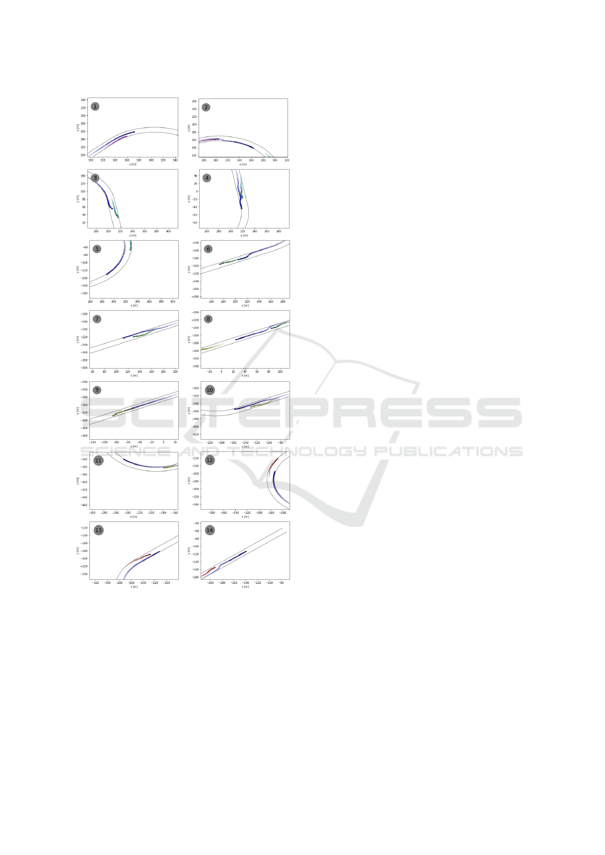
Figure 10: Computed trajectories for a test scenario on the
track.
4 CONCLUSION
In this manuscript, we discussed the advantages and
disadvantages of data based and classical optimal
control techniques. We combined these two worlds
such that the disadvantages are suppressed and the ad-
vantages are highlighted. In the hierarchical structure,
RL tackles the collision avoidance problem, which
posed problems for the classical methods. The other
way round, we apply a classical technique in order to
actually steer the dynamical system, which we know
from its equations of motion. We have seen that we
can accelerate the training and the control genera-
tion of the final controller by a surrogate model, if
the optimal control problem, although it is much eas-
ier without collision avoidance constraints, takes too
much time to be solved. We successfully applied this
strategy to our maneuvers on a racing track. We were
able to follow a given course and thereby avoid sev-
eral moving obstacles, which were driving randomly
on the street. We showed that we were able to find a
fast controller for planning collision free paths.
From our point of view, these results are promis-
ing for more complex scenarios and real world appli-
cations. We are sure that the above approach can, for
instance, be of even greater value in the field of dock-
ing maneuver in space, where the complexity of the
dynamical system (e.g. satellite) as well as the com-
plexity of the shape, which needs to be considered for
collision avoidance, are significantly higher. In the
case of autonomous driving, the long time goal is the
implementation on a real world car.
ACKNOWLEDGEMENTS
The authors are grateful for the funding by the Fed-
eral Ministry of Education and Research of Germany
(BMBF), project number 05M20WNA (SOPRANN).
Furthermore, this research has been conducted within
the project frame of SeRANIS – Seamless Radio Ac-
cess Networks in the Internet of Space. The project
is funded by dtec.bw – Digitalization and Technol-
ogy Research Center of the Bundeswehr. dtec.bw is
funded by the European Union-Next Generation EU.
REFERENCES
Abadi, M., Agarwal, A., Barham, P., Brevdo, E., Chen, Z.,
Citro, C., Corrado, G. S., Davis, A., Dean, J., Devin,
M., Ghemawat, S., Goodfellow, I., Harp, A., Irving,
G., Isard, M., Jia, Y., Jozefowicz, R., Kaiser, L., Kud-
lur, M., Levenberg, J., Man
´
e, D., Monga, R., Moore,
S., Murray, D., Olah, C., Schuster, M., Shlens, J.,
Steiner, B., Sutskever, I., Talwar, K., Tucker, P., Van-
houcke, V., Vasudevan, V., Vi
´
egas, F., Vinyals, O.,
Warden, P., Wattenberg, M., Wicke, M., Yu, Y., and
Zheng, X. (2015). TensorFlow: Large-scale machine
learning on heterogeneous systems. Software avail-
able from tensorflow.org.
Attia, A. and Dayan, S. (2018). Global overview of imita-
tion learning.
VEHITS 2024 - 10th International Conference on Vehicle Technology and Intelligent Transport Systems
86

Banerjee, C., Nguyen, K., Fookes, C., and Raissi, M.
(2023). A survey on physics informed reinforcement
learning: Review and open problems.
Bellman, R. E. (1957). Dynamic Programming. Princeton
University Press, Princeton, NJ, USA, 1 edition.
Bertsekas, D. (2019). Reinforcement Learning and Optimal
Control. Athena Scientific optimization and computa-
tion series. Athena Scientific.
de Boor, C. (1978). A practical guide to splines. In Applied
Mathematical Sciences.
De Marchi, A., Dreves, A., Gerdts, M., Gottschalk, S., and
Rogovs, S. (2022). A function approximation ap-
proach for parametric optimization. Journal of Op-
timization Theory and Applications. in press.
Deuflhard, P. (2011). Newton Methods for Nonlinear Prob-
lems: Affine Invariance and Adaptive Algorithms.
Springer Publishing Company, Incorporated.
Feinberg, E. A. and Shwartz, A. (2002). Handbook of
Markov Decision Processes: Methods and Applica-
tions. International Series in Operations Research.
Springer US.
Feng, S., Sebastian, B., and Ben-Tzvi, P. (2021). A colli-
sion avoidance method based on deep reinforcement
learning. Robotics, 10(2).
Fischer, A. (1992). A special newton-type optimization
method. Optimization, 24:269–284.
Gerdts, M. (2024). Optimal Control of ODEs and DAEs.
De Gruyter Oldenbourg, Berlin, Boston, 2 edition.
Gottschalk, S. (2021). Differential Equation Based Frame-
work for Deep Reinforcement Learning. Dissertation.
Fraunhofer Verlag.
Gr
¨
une, L. and Junge, O. (2008). Gew
¨
ohnliche Differential-
gleichungen. Springer Studium Mathematik - Bache-
lor. Springer Spektrum Wiesbaden, 2 edition.
Ito, K. and Kunisch, K. (2009). On a semi-smooth newton
method and its globalization. Mathematical Program-
ming, (118):347–370.
Karush, W. (1939). Minima of Functions of Several Vari-
ables with Inequalities as Side Conditions. Dis-
sertation. Department of Mathematics, University of
Chicago, Chicago, IL, USA.
Kingma, D. and Ba, J. (2014). Adam: A method for
stochastic optimization. International Conference on
Learning Representations.
Kuhn, H. W. and Tucker, A. W. (1951). Nonlinear pro-
gramming. In Proceedings of the Second Berkeley
Symposium on Mathematical Statistics and Probabil-
ity, pages 481–492, Berkeley, CA, USA. University of
California Press.
Landgraf, D., V
¨
olz, A., Kontes, G., Mutschler, C., and
Graichen, K. (2022). Hierarchical learning for model
predictive collision avoidance. IFAC-PapersOnLine,
55(20):355–360. 10th Vienna International Confer-
ence on Mathematical Modelling MATHMOD 2022.
Liniger, A., Domahidi, A., and Morari, M. (2015).
Optimization-based autonomous racing of 1:43 scale
rc cars. Optimal Control Applications and Methods,
36:628–647.
Lot, R. and Biral, F. (2014). A curvilinear abscissa approach
for the lap time optimization of racing vehicles. IFAC
Proceedings Volumes, 47(3):7559–7565. 19th IFAC
World Congress.
Moerland, T. M., Broekens, J., Plaat, A., and Jonker, C. M.
(2020). Model-based reinforcement learning: A sur-
vey.
Pagot, E., Piccinini, M., and Biral, F. (2020). Real-time op-
timal control of an autonomous rc car with minimum-
time maneuvers and a novel kineto-dynamical model.
IEEE International Conference on Intelligent Robots
and Systems, pages 2390–2396.
Pateria, S., Subagdja, B., Tan, A., and Quek, C. (2021). Hi-
erarchical reinforcement learning: A comprehensive
survey. ACM Comput. Surv., 54(5).
Ramesh, A. and Ravindran, B. (2023). Physics-informed
model-based reinforcement learning.
Reid, M. D. and Ryan, M. R. K. (2000). Using ilp to im-
prove planning in hierarchical reinforcement learning.
In ILP.
Rumelhart, D. E., Hinton, G. E., and Williams, R. J. (1986).
Learning Representations by Back-propagating Er-
rors. Nature, 323:533–536.
Schulman, J., Levine, S., Abbeel, P., Jordan, M. I., and
Moritz, P. (2015). Trust region policy optimization.
In ICML, volume 37 of JMLR Workshop and Confer-
ence Proceedings, pages 1889–1897. JMLR.org.
Silver, D., Lever, G., Heess, N., Degris, T., Wierstra, D.,
and Riedmiller, M. (2014). Deterministic policy gra-
dient algorithms. In Xing, E. P. and Jebara, T., edi-
tors, Proceedings of the 31st International Conference
on Machine Learning, volume 32 of Proceedings of
Machine Learning Research, pages 387–395, Bejing,
China. PMLR.
Sussmann, H. and Willems, J. (1997). 300 years of optimal
control: from the brachystochrone to the maximum
principle. IEEE Control Systems Magazine, 17(3):32–
44.
Sutton, R. S. and Barto, A. G. (2018). Reinforcement Learn-
ing: An Introduction. The MIT Press, second edition.
Williams, R. J. (1992). Simple statistical gradient-following
algorithms for connectionist reinforcement learning.
Machine Learning, 8:229–256.
Wischnewski, A., Herrmann, T., Werner, F., and Lohmann,
B. (2023). A tube-mpc approach to autonomous multi-
vehicle racing on high-speed ovals. IEEE Transac-
tions on Intelligent Vehicles, 8(1):368–378.
Reinforcement Learning and Optimal Control: A Hybrid Collision Avoidance Approach
87