Using Deep Learning for the Dynamic Evaluation of Road Marking

Features from Laser Imaging

Maxime Tual, Val

erie Muzet

, Philippe Foucher

, Christophe Heinkel

and Pierre Charbonnier

Research Team ENDSUM, Cerema, 11 rue Jean Mentelin, 67035 Strasbourg, France

Keywords:

Road Marking, Deep Learning, Regression, Evaluation, Laser Data, LCMS Sensor.

Abstract:

Road markings are essential guidance elements for both drivers and driver assistance systems: their mainte-

nance requires regularly scheduled performance surveys. In this paper, we introduce a deep learning based

method to estimate two indicators of the quality of road markings (the percentage of remaining marking and

the contrast) directly from their appearance, using reﬂectance data acquired by a mobile laser imaging system

used for inspections. To do this, we enhance the EfﬁcientDet architecture by adding an output sub-network to

predict the indicators. It is not possible to physically establish large-scale reference measurements for train-

ing and testing our model, but this can be done indirectly by semi-supervised image annotation, a strategy

validated by our experiments. Our results show that it is advisable to train the model end-to-end without op-

timizing its detection performance. They also enlighten the very good accuracy of the indicators predicted by

the model.

1 INTRODUCTION

In this contribution, we introduce a method, based on

an end-to-end trainable deep learning model, for eval-

uating quality metrics directly from the visual appear-

ance of road markings, as illustrated in ﬁg. 1.

Figure 1: Our method provides a bounding box surround-

ing the marking, and an estimate of its quality, without any

intermediate processing.

Road markings provide both visibility and visual

guidance to the driver and, nowadays, to advanced

driver assistance systems (ADAS) and autonomous

vehicles. Maintaining markings in good condition is

therefore fundamental for road safety, and this implies

regular inspections. To carry out measurements of

marking quality, we consider here two complemen-

tary metrics, that are related to the visual quality of

markings in daytime, namely the percentage of resid-

https://orcid.org/0000-0002-0026-6592

https://orcid.org/0000-0003-1218-636X

https://orcid.org/0000-0002-3532-393X

https://orcid.org/0000-0002-9374-5647

ual marking (PRM), which characterizes the level of

wear of the paint itself, and the contrast between the

remaining painted surface and the surrounding pave-

ment.

In this work, we use a laser imaging system, po-

sitioned vertically to the road. It provides an image

of the intensity reﬂected from the pavement and the

markings, independent of the external conditions, in a

geometry favorable to PRM and contrast estimation.

Whereas many methods have been developed over

the last decades to detect road markings for vehicle

guidance purposes, few works have been concerned

with the evaluation of the quality of markings from

images. The commonly used approach is to perform

a segmentation of the markings (i.e. to estimate a map

of pixel membership to the marking) and to compute

the metrics from it. The drawback of this approach

is that it usually involves setting a series of parame-

ters, and that errors can propagate from one process-

ing step to the next, with a strong impact on the ﬁnal

result.

We postulate that segmentation is not necessary,

and that it should be possible to infer the quality mea-

sures of the marking directly from the images. This

is a regression task, certainly highly dimensional and

non-linear, but which deep learning techniques are

nowadays able to handle. Of course, it is necessary

Tual, M., Muzet, V., Foucher, P., Heinkelé, C. and Charbonnier, P.

Using Deep Learning for the Dynamic Evaluation of Road Marking Features from Laser Imaging.

DOI: 10.5220/0012595600003720

Paper published under CC license (CC BY-NC-ND 4.0)

In Proceedings of the 4th International Conference on Image Processing and Vision Engineering (IMPROVE 2024), pages 23-31

ISBN: 978-989-758-693-4; ISSN: 2795-4943

to locate in the image the marking element that corre-

sponds to a given measurement, surrounding it with a

bounding box. This is a detection task, another prime

application for deep learning.

We have therefore modiﬁed an efﬁcient neural ar-

chitecture dedicated to object detection in images, by

adapting it to the case of road markings and by adding

a sub-network allowing the inference of the sought in-

dicators. To carry out the training of this composite

network and the evaluation of its predictions, a large

quantity of images was collected and annotated by an

operator in a semi-supervised fashion. We show the

promising results obtained by this novel method.

The rest of the paper is organized as follows. In

sec. 2, we propose a brief review of existing related

works. Then, we describe in sec. 3 how we collected

the data needed to train and evaluate our method.

Sec. 4 is dedicated to methodological aspects related

to the annotation of markings, the architecture of the

proposed deep learning model and its training. Ex-

perimental results are presented in sec. 5, and sec. 6

concludes the paper.

2 RELATED WORK

In this paper, we aim at evaluating the visual qual-

ity of the markings, with characteristics that can

be related to the performance of both human vi-

sion and automated vehicle (AV) systems, in day-

light. It was shown that the contrast between mark-

ing and surrounding road surface is a good candidate

for this (Carlson and Poorsartep, 2017) and there-

fore it is one of our parameters of interest. We

moreover consider the percentage of residual marking

(PRM), which also conditions the visibility of mark-

ings. Even if the latter is deﬁned in several coun-

tries, like UK (CS 126, 2022), Korea (Lee and Cho,

2023), Germany (Mesenberg, 2003) and France (NF

EN 1824, 2020), it often appears in the form of

a score, quantized according to wear level classes,

called cover index. Moreover, the standardized mea-

surement geometry (2.29

◦

observation angle) is too

grazing to evaluate it precisely and, to our knowledge,

there is no operational PRM measurement system, un-

til now. We propose an answer to this need, thanks

to an imaging device that acquires images at trafﬁc

speed, under a 90

◦

angle, and to a method that esti-

mates a PRM ﬁgure, not a wear level class.

Road marking detection has been investigated for

more than 40 years with the aim of designing ADAS,

in particular lane keeping systems: a complete survey

of the topic is therefore out of the scope of this pa-

per. Note that processing methods have been devel-

oped for passive acquisition systems (supplying im-

ages) (Zhang et al., 2022) as well as for active ones

(using laser scanners or retroreﬂectometers) (Zhang

et al., 2019). The system we use is active, which al-

lows getting rid of illumination variations (e.g. shad-

ows) and therefore, to obtain infrastructure-intrinsic

measurements.

Earlier methods (see e.g. (Bar Hillel et al., 2014)

for a survey) used an algorithmic approach in which,

typically, putative marking elements are ﬁrst extracted

from the images by global thresholding (a great clas-

sic is the Otsu method), or by local thresholding and

geometric selection (Veit et al., 2008). Then, curves

are ﬁtted to the detections in a robust manner, for ex-

ample using the Hough transform (Em et al., 2019) or

M-estimators (Tarel et al., 2002), to model marking

lines. Although these methods have made it possible

to drive vehicles automatically for a long time, they

involve adjusting many parameters and their detec-

tion performances have now been largely surpassed

by those of deep learning methods.

Deep learning approaches, based on convolutional

neural networks (CNNs), require the annotation of a

huge number of markings on images, which can be

very time consuming. We propose automatisms, im-

plemented in an ergonomic graphical user interface,

which provide a non-negligible help to the operator.

Once the CNN has been trained from the annotated

images, it can be used to detect the road markings and

then, to model the marking lines, see e.g. (Liang et al.,

2020; Zhang et al., 2022).

All the above methods are dedicated to the detec-

tion of road markings. Among the few publications

that deal with the evaluation of road markings, we can

cite (Lee and Cho, 2023), where a Mask R-CNN (He

et al., 2017) model is applied to detect the markings

in the image. Then, Otsu thresholding is used to seg-

ment it and a quality measure, that appears to be the

complement to one of the PRM, is computed. Using

the Otsu method for segmentation seems to us some-

what incomprehensible, since Mask R-CNN is an in-

stance segmentation algorithm and, as such, already

provides a segmentation. In (Soil

an et al., 2022), the

intensity of laser scanning data is processed to evalu-

ate the performance of road markings and to relate it

to retroreﬂection (the standard measurement of mark-

ing quality of use in night conditions). The process

involves a segmentation of the markings, but no de-

tails on this step are given in the paper. We note that

both approaches include a segmentation step, which

we do not consider necessary to estimate the quality

measure of the marking from its visual appearance.

IMPROVE 2024 - 4th International Conference on Image Processing and Vision Engineering

3 EXPERIMENTAL SETUP

3.1 LCMS Sensor

The vehicle used for experiments, shown on ﬁg. 2,

was developed to monitor road pavement degradation

on the French national network. It is equipped with a

pair of high resolution LCMS (Laser Crack Measure-

ment System) sensors developed by the Pavemetrics

company (Laurent et al., 2014). Each LCMS sensor is

made of a laser which emits a line to the road surface,

and of a linear camera that records the deformation

and the intensity of the reﬂected signal. The resulting

1D depth and intensity proﬁles are stacked to gener-

ate couples of 2D images. In our experiments, points

are acquired every 1 mm for each proﬁle and proﬁles

are acquired every 5 mm. In this study, the focus is on

intensity, which corresponds to a retroreﬂected sig-

nal with both an emission and an observation angle of

◦

, a geometry well suited to the estimation of PRM.

The signal is quantized into 256 gray levels, a spatial

equalization preprocessing is applied and the images

from the two sensors are merged to cover the entire

width of the lane (see example in ﬁg. 5).

Figure 2: Picture of Aigle3D, with its 4 m measuring swath

depicted in green.

3.2 Experimental Sites and Datasets

Five experimental campaigns were carried out to ac-

quire the whole LCMS data. Quantitative and quali-

tative information on the recorded datasets is summa-

rized in table 1. Note that the ﬁrst two experiments

(named Satory and Satory-2023) took place in a con-

ﬁned test site. In order to simulate different levels

of marking wear in a controlled way, stencils were

used (see ﬁg. 3), which provides a physical reference

for PRM. The other three acquisition campaigns took

place on open roads. We have selected different types

of roads with relatively varied marking conditions,

and such that the most usual road marking modules

are represented in the database.

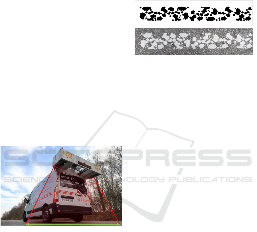
Figure 3: Sample stencil (top) producing a road marking

with 45% PRM.

4 METHODOLOGY

4.1 Annotation

The model to be trained aims at providing the PRM

and contrast for each detected marking. These metrics

must therefore be previously known for every mark-

ing of the training and testing datasets. As explained

in section 3.2, some stencils can be used to imple-

ment markings with known PRM. Such direct, physi-

cal PRM reference can be made available for a few

dozen examples on conﬁned roads (e.g. in Satory,

we have PRMs of about 23%, 41% and 100%) but

this strategy cannot be implemented on a large-scale

on open roads. For this reason, we have developed

an approach that computes PRM and contrast indirect

reference measures using image processing methods

as follows:

1. The operator selects manually in the image an

area with a road marking (see ﬁg. 4-A);

2. Image binarization (marking/non-marking) is per-

formed based on a gaussian mixture modeling

(GMM) of pixel intensities: the component with

highest mean is selected as marking. Mathemati-

cal Morphology tools are then applied either to re-

move small connected components (opening oper-

ation) or to ﬁll in small holes in the region (closure

operation). The resulting black and white image

is shown in ﬁg. 4-B;

3. The different connected components correspond-

ing to a same marking are manually merged to

provide a single connected component (see ﬁg. 4-

C);

4. The segmentation is divided into k rectangles (k

chosen by the user), as shown in ﬁg. 4-D. For

each part, the rectangle minimizing the surface

area that contains the contour points is selected;

Using Deep Learning for the Dynamic Evaluation of Road Marking Features from Laser Imaging

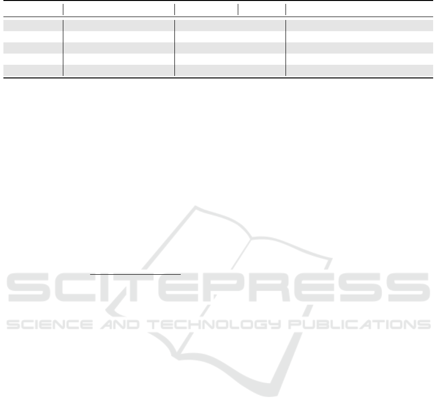
Table 1: Description of the LCMS datasets.

Name Road type Length (km) # images Comments

Satory Closed test site 1.7 71 Physical references (stencils)

Satory-2023 Closed test site 1.5 50 Physical references (more stencils)

Site 2 Major roads 14.0 619 Markings in fairly good condition

Site 3 Urban road 8.5 709 Markings in fairly good condition

Rouen area Urban & secondary roads 37.0 1203 Markings in varying conditions

5. The union of all rectangles deﬁnes the polygo-

nal envelope of the marking. The polygon is

smoothed to obtain a uniform marking width

along the entire length. The ﬁnal envelope is rep-

resented in orange in ﬁg. 4-E. The blue rectangu-

lar box, parallel to image axis, is the bounding box

used as ground truth for the training;

6. The PRM is computed as the ratio between the to-

tal number of pixels considered as road marking

within the orange envelope and the area of the en-

velope;

7. Considering the orange envelope area, a maximal

contrast ratio is also computed between the mark-

ing and the surrounding pavement:

Contrast =

marking

min(I

RoadU p

, I

RoadDown

)

(1)

where I

marking

is the mean intensity of the seg-

mented marking and I

RoadU p

(resp. I

RoadDown

) is

the average intensity of the pavement above (resp.

below) the marking, on a surface equal to that of

the envelope.

It should be observed that this approach requires

several operator-machine interactions. We use a mod-

iﬁed version of the S3A software (Jessurun et al.,

2020) in which we have integrated our own func-

tionalities for helping the operator in these tasks (see

ﬁg. 5). In the upper part of the interface the processed

image is displayed, surrounded by two panels for set-

ting the visualization and processing parameters. The

lower part displays the images at a larger scale (along

a route). The annotated marking lines are displayed

in color, with one color per marking typology, and the

image being processed highlighted in blue. Note that

image annotation and calculation of reference values

for PRM and contrast are performed on full resolution

images.

4.2 Modiﬁed EfﬁcientDet Architecture

We propose a modiﬁed version of EfﬁcientDet (Tan

et al., 2020), a one-stage object detection network.

This architecture is at least as efﬁcient as other con-

volutional networks dedicated to object detection, but

involves much less parameters. The modiﬁed archi-

tecture is shown in ﬁg. 6. We use the backbone Ef-

ﬁcientNetv2, proposed in (Tan and Le, 2021) for our

implementation. It is a bottom-up network that ex-

tracts features from the highest to the lowest spa-

tial resolution. In the classical Feature Pyramid Net-

work (FPN) (Lin et al., 2017a), feature maps are pro-

gressively upsampled as higher resolutions, in a top-

down pathway, where skip-connections are used to

directly re-introduce semantic information from the

backbone feature map at the same resolution. In Ef-

ﬁcientDet, the authors propose a bi-directional Fea-

ture Pyramid Network (see biFPN layer in ﬁg. 6), in

which multi-scale feature maps are merged in both a

top-down and a bottom-up ﬂow so as to achieve a bet-

ter cross-scale feature network topology with limited

extra cost. In the original EfﬁcientDet architecture,

prediction heads are composed of two sub-networks.

In the original EfﬁcientDet architecture, the pre-

diction heads are composed of two sub-networks. The

classiﬁcation network identiﬁes the category of the

detected object and provides a conﬁdence score. In

our case, this head is adapted to binary classiﬁcation:

marking or non-marking. The bounding box network

provides the position and size of the rectangle delim-

iting the object of interest. In this contribution, we

propose to add a third sub-network to this architec-

ture, namely the indicator net (see ﬁg. 6), that imple-

ments a regression model to assess both the PRM and

contrast values of the detected markings directly. This

provides a visual assessment of marking quality.

In our modiﬁed EfﬁcientDet model, the overall

loss function to be minimized is deﬁned as:

L = L

class

+ L

bbox

+ L

indicator

(2)

where L

class

, used to train the classiﬁcation sub-

network, is a focal loss (Lin et al., 2017b), with pa-

rameters γ = 1.5 and α = 0.25. The regression mod-

els for bounding box and indicators nets are trained

by minimizing L

bbox

and L

indicator

, respectively. Both

are Huber losses with parameter δ = 0.1.

IMPROVE 2024 - 4th International Conference on Image Processing and Vision Engineering

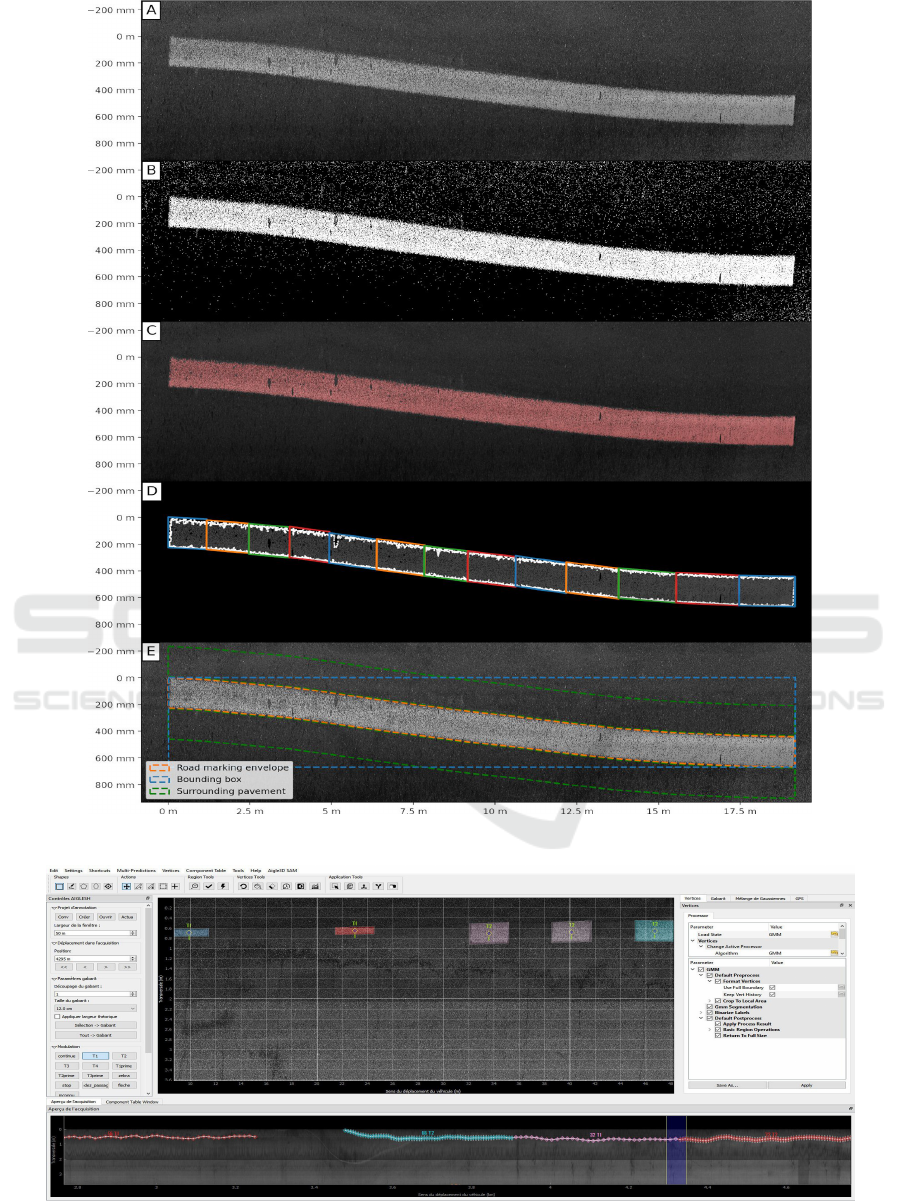
Figure 4: Illustration of the annotation pipeline (the deformation of the marking is exaggerated by the non-uniform scaling).

Figure 5: Illustration of the annotation software (better visualized in the digital version).

Using Deep Learning for the Dynamic Evaluation of Road Marking Features from Laser Imaging

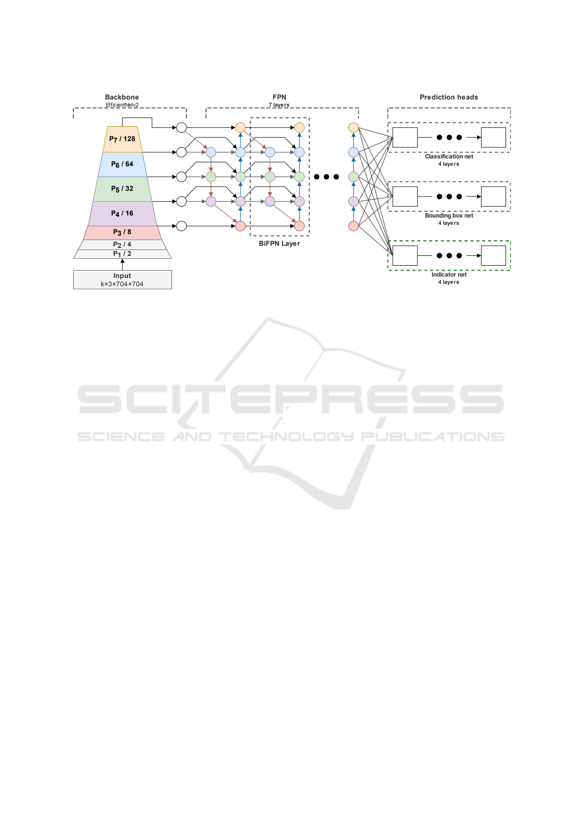
Figure 6: Our modiﬁed version of EfﬁcientDet. The additional sub-network (indicator net) appears in the green rectangle.

4.3 Training Protocol

We train our model by transfer learning from the

weights issued from EfﬁcientNetv2, itself trained on

ImageNet-1k dataset (Tan and Le, 2021). As is cus-

tomary in this type of ﬁne-tuning process, we opti-

mize the parameters of the components of the model

(backbone, biFPN and prediction heads) according to

a sequential protocol: ﬁrst we specialize the model

for the application by freezing the backbone (hence

the feature extractor parameters) and training the rest

of the architecture, then we release all parameters and

train them, ﬁnally, we reﬁne the model by repeating

the ﬁrst step. More speciﬁcally, we tested three vari-

ants of this strategy, described in table 2, leading to

three models whose prediction performance will be

discussed in subsection 5.3.

In the ﬁrst protocol (leading to model A), we ﬁrst

train our architecture as a classical EfﬁcientDet, i.e.

optimizing solely its detection components (classiﬁ-

cation and bounding box nets), and only then do we

proceed with the separate training of the additional

head in charge of indicator estimation (indicator net).

In the third protocol (leading to model C), we opti-

mize the entire proposed architecture, end-to-end. Fi-

nally, the second protocol (leading to model B) is an

intermediate strategy, which starts like strategy A and

ends like strategy C.

Note that, in order to be consistent with the

3-component image format used in the pretrained

model (Tan and Le, 2021), we had to replicate two

times the single intensity component of LCMS im-

ages. Using the full resolution images of 4160×4000

would have required great time and computation re-

source, so we downsize the images by a factor of

about 6. Tests have shown that the impact of this sub-

sampling on the PRM is about 2.6%. Finally, in order

to accommodate the great number of images required

to train deep learning models, we use geometric data

augmentations during training. Morespeciﬁcally, im-

ages are randomly scaled with a factor between 0.75

and 1.5, rotated with an angle between −10° and 10°,

shifted by a displacement between −10% and 10%,

then cropped and zero padded into a 704 × 704 pixel

image.

5 RESULTS

5.1 Reference PRM Evaluation

As mentioned in sec. 4.1, the PRM and contrast ref-

erence values used for training and testing the indi-

cator net are indirect, in that they are established by

image processing during the annotation. However, a

physical reference value is available for markings im-

planted with stencils of known PRM. We used them

to evaluate the indirect referencing process. For ex-

ample, on two populations of 48 annotated markings

with a theoretical (stencil) PRM of 23%, we obtained

24.52% and 24.50% mean PRM with standard devia-

tions of 2.06% and 3.45%, respectively. Likewise, on

2 × 48 annotated markings with a theoretical PRM of

41%, we obtained a mean PRM of 40.97% and 41.4%

with standard deviations of 4.95% and 3.55%. Finally

all new markings with a 100% theoretical PRM were

evaluated. The mean is 99.97% with standard devia-

tion of 0.101%. These experiences give a clear indica-

IMPROVE 2024 - 4th International Conference on Image Processing and Vision Engineering

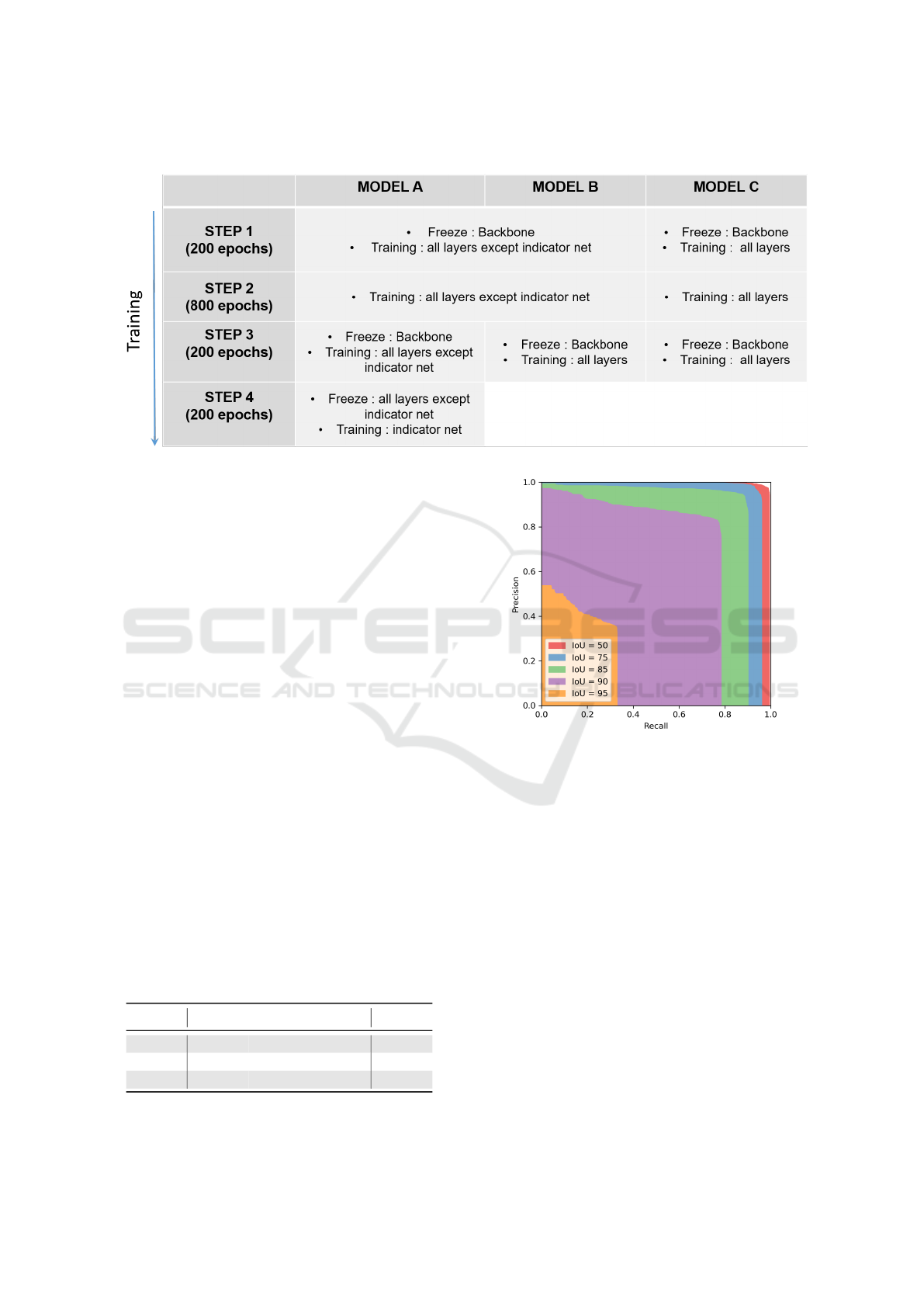
Table 2: Deﬁnition of training strategies.

tion of the quality of our indirect referencing method-

ology.

5.2 Detection Evaluation

Models are trained from the 1893 images of the

datasets Satory, Site 2 and Rouen Area (see table 1).

We split the database in 80% images for training and

20% for validation. Due to the limited number of im-

ages available, a ﬁve-fold cross-validation (CV) pro-

cedure is performed to train and evaluate the global

performance of algorithm.

We ﬁrst evaluate the performance of models A,

B and C in terms of detection quality. To this aim,

we use all the images in dataset Site 3. We con-

sider a true positive detection if the overlap between

predicted and ground truth bounding boxes, deﬁned

by the intersection-over-union (IoU) metric, is over a

given threshold Θ. For each value of Θ, a Precision-

Recall (P-R) curve can be plot by varying the detec-

tion threshold and computing the precision as the pro-

portion of true positive predictions among all predic-

tions and the recall, as the proportion of positives suc-

cessfully detected. The area under the P-R curve is the

average precision, AP

. Finally, the average of AP

computed for Θ ∈ {50, 55, 60, ..., 95}% is denoted by

AP (average precision).

Table 3: Detection results for the different models (see text).

Model AP

A 0.9890 0.9481 0.1456 0.8432

B 0.9905 0.9474 0.1236 0.8371

C 0.9800 0.8759 0.0508 0.7457

Figure 7: P-R curve for Model B (CV test subset #2). The

ﬁgures in table 3 correspond to the area under the

curves (displayed in colors).

Fig. 7 shows examples of P-R curves obtained

with model B, on one of the test subsets and table 3

summarizes the mean performance of the three evalu-

ated models over the ﬁve CV subsets (we observed

homogeneous performance over the subsets). One

may see that AP

decreases with Θ (and even falls for

Θ = 95%). A visual screening of the results showed

us that the bounding boxes provided by our models

have a slight tendency to be overestimated, which can

be partly explained by the way we handle the rotations

in the data augmentation step at at learning time. We

are planning modiﬁcations that should allow us to im-

prove this. Finally, we note that models A and B per-

form better than model C in detection, which is con-

sistent with the fact that the former are issued from an

optimization strategy favoring detection over param-

eter regression.

Using Deep Learning for the Dynamic Evaluation of Road Marking Features from Laser Imaging

5.3 Quality Indicator Evaluation

We now evaluate the predictions of the PRM and con-

trast by our three learned models against the corre-

sponding indirect references. The provided statis-

tics, namely root-mean-squared differences (RMSD),

mean difference (Bias), standard deviations (STD),

median difference (Med), Median Absolute Deviation

(MAD), ﬁrst and ninth decile of differences are aver-

ages resulting from cross-validation. We use as the

IoU threshold a value of Θ = 75%, which we have

found to provide a good compromise between the re-

quirement for detection accuracy and the quality of

the predicted PRM and contrast measurements. The

results are shown in table 4 for the PRM and in ta-

ble 5 for the contrast. As can be seen, model C is the

one that provides the best results for the PRM. For

the contrast, models B and C provide about the same

performance, better than model A. This experiment

conﬁrms that it is more suitable to train the model di-

rectly, without trying to optimize the quality of the

detection ﬁrst.

Table 4: Statistics of PRM differences between ground truth

and model predictions, with IoU = 75%.

Model RMSD Bias STD Med MAD Q10 Q90

A 10.92 -3.02 10.44 -3.34 6.15 -15.55 9.60

B 7.80 -0.10 7.78 -0.84 3.70 -8.41 9.08

C 6.70 -0.86 6.61 -1.30 3.12 -8.11 6.99

Table 5: Statistics of contrast differences with IoU = 75%

(contrast values lie between 1.5 and 8.9 in the test dataset).

Model RMSD Bias STD Med MAD Q10 Q90

A 1.21 -0.39 1.15 -0.06 0.45 -1.96 0.60

B 0.71 -0.27 0.66 -0.13 0.25 -1.03 0.32

C 0.72 -0.27 0.67 -0.13 0.25 -1.04 0.34

Table 6: Statistics of PRM differences between model pre-

dictions and physical reference.

Model RMSD BIAS STD Med MAD Q10 Q90

A 17.23 2.11 17.22 0.06 13.15 -20.79 25.69

B 7.16 1.84 6.37 1.83 5.09 -6.05 10.24

C 6.16 2.12 5.41 2.09 3.93 -4.78 8.41

Finally, it is desirable to evaluate the quality of the

PRM regression against physical references. To this

end, we recently conducted a new acquisition cam-

paign on a stencil-marked site (Satory-2023, see Ta-

ble 1), using seven PRM reference values (approxi-

mately 25, 45, 56, 65, 74, 80 and 100%), but on a

limited number of samples (8 per PRM value). The

statistics in Table 6 show that model C gives the best

performance, and that the differences are quite small

(around 2%, with a dispersion around 5%). Careful

examination of the results, however, shows that the

bias is greater for low PRM values than for values

above 50%. This result is consistent with the statis-

tics of our training dataset, where worn-out markings

are underrepresented.

6 CONCLUSIONS

In this paper, we have proposed an innovative method

for assessing the quality of road markings, which

could facilitate their inspection. More speciﬁcally, we

have proposed a neural architecture that enables esti-

mating two indicators of road marking quality (Per-

centage of Remaining Marking and contrast), directly

from their visual appearance.

It is not possible to build, at least not on a large

scale, a physical reference for these measurements

and one must thus resort to an indirect reference com-

puted by image processing at annotation time. The

experimental results we report show the validity of

using an indirect reference.

Experimental results also show that it is possible

to correctly estimate road marking quality indicators

directly from their visual appearance, using a properly

trained neural network, without the need for prior seg-

mentation. Moreover, at training time, it is not neces-

sary to separately optimize the detection part of our

architecture: it can be trained directly end-to-end by

ﬁne-tuning from a pre-trained model.

Lastly, preliminary results from new experimen-

tal measurements (with a limited number of samples,

however) suggest excellent agreement between pre-

dicted PRM and physical reference values. We be-

lieve that these results can be further enhanced by im-

proving some points of the training procedure, as well

as by increasing the corpus of data, paying particular

attention to poor quality markings.

ACKNOWLEDGEMENTS

This work received ﬁnancial support of the ADEME

French project SAM (Safety and Acceptability of Au-

tonomous Mobility), funding number 1982C0034.

REFERENCES

Bar Hillel, A., Lerner, R., Levi, D., and Raz, G. (2014).

Recent progress in road and lane detection: a survey.

Machine vision and applications, 25(3):727–745.

Carlson, P. J. and Poorsartep, M. (2017). Enhancing the

Roadway Physical Infrastructure for Advanced Vehi-

IMPROVE 2024 - 4th International Conference on Image Processing and Vision Engineering

cle Technologies: A Case Study in Pavement Mark-

ings for Machine Vision and a Road Map Toward

a Better Understanding. In Transportation Research

Board 96th Annual Meeting. Number: 17-06250.

CS 126 (2022). Inspection and assessment of road markings

and road studs. Dmrb, Highways England: Guild-

ford, UK; Transport Scotland: Edinburgh, UK; Lly-

wodraeth Cymru Welsh Government: Cardiff.

Em, P. P., Hossen, J., Fitrian, I., and Wong, E. K. (2019).

Vision-based lane departure warning framework. He-

liyon, 5(8):e02169.

He, K., Gkioxari, Doll

ar, P., and Girshick, R. a. (2017).

Mask R-CNN. In IEEE International Conference on

Computer Vision (ICCV), pages 2980–2988.

Jessurun, N., Paradis, O., Roberts, A., and Asadizanjani, N.

(2020). Component detection and evaluation frame-

work CDEF): A semantic annotation tool. Microscopy

and Microanalysis, 26(S2):1470–1474.

Laurent, J., H

ebert, J. F., Lefebvre, D., and Savard, Y.

(2014). 3D laser road proﬁling for the automated mea-

surement of road surface conditions and geometry. In

17th International Road Federation World Meeting,

volume 2, page 30.

Lee, S. and Cho, B. H. (2023). Evaluating Pavement

Lane Markings in Metropolitan Road Networks with

a Vehicle-Mounted Retroreﬂectometer and AI-Based

Image Processing Techniques. Remote Sensing,

15(7):1812.

Liang, D., Guo, Y.-C., Zhang, S.-K., Mu, T.-J., and Huang,

X. (2020). Lane Detection: A Survey with New Re-

sults. Journal of Computer Science and Technology,

35(3):493–505.

Lin, T.-Y., Doll

ar, P., Girshick, R., He, K., Hariharan, B.,

and Belongie, S. (2017a). Feature pyramid networks

for object detection. In IEEE conference on computer

vision and pattern recognition, pages 2117–2125.

Lin, T.-Y., Goyal, P., Girshick, R., He, K., and Doll

ar, P.

(2017b). Focal loss for dense object detection. In

IEEE international conference on computer vision,

pages 2980–2988.

Mesenberg, H.-H. (2003). Ztv m 02: Die neuen

zus

atzlichen technischen vertragsbedingungen und

richtlinien f

ur markierungen auf straßen. German reg-

ulation, BAST.

NF EN 1824 (2020). Road marking materials - road trials.

French standard, CEN.

Soil

an, M., Gonz

alez-Aguilera, D., del Campo-S

anchez,

A., Hern

andez-L

opez, D., and Del Pozo, S. (2022).

Road marking degradation analysis using 3D point

cloud data acquired with a low-cost Mobile Mapping

System. Automation in Construction, 141:104446.

Tan, M. and Le, Q. (2021). EfﬁcientNetv2: Smaller mod-

els and faster training. In International conference on

machine learning, pages 10096–10106. PMLR.

Tan, M., Pang, R., and Le, Q. V. (2020). EfﬁcientDet:

Scalable and Efﬁcient Object Detection. In 2020

IEEE/CVF Conference on Computer Vision and Pat-

tern Recognition (CVPR).

Tarel, J.-P., Ieng, S.-S., and Charbonnier, P. (2002). Us-

ing robust estimation algorithms for tracking explicit

curves. In 7th European Conference on Computer Vi-

sion (ECCV), pages 492–407.

Veit, T., Tarel, J.-P., Nicolle, P., and Charbonnier, P. (2008).

Evaluation of Road Marking Feature Extraction. In

11th International IEEE Conference on Intelligent

Transportation Systems, pages 174–181.

Zhang, D., Xu, X., Lin, H., Gui, R., Cao, M., and He, L.

(2019). Automatic road-marking detection and mea-

surement from laser-scanning 3D proﬁle data. Au-

tomation in Construction, 108:102957.

Zhang, Y., Lu, Z., Zhang, X., Xue, J.-H., and Liao, Q.

(2022). Deep Learning in Lane Marking Detection: A

Survey. IEEE Transactions on Intelligent Transporta-

tion Systems, 23(7):5976–5992.

Using Deep Learning for the Dynamic Evaluation of Road Marking Features from Laser Imaging