Improving Explainability of the Attention Branch Network with CAM

Fostering Techniques in the Context of Histological Images

Pedro Lucas Miguel

, Alessandra Lumini

2 a

, Giuliano Cardozo Medalha

, Guilherme F. Roberto

4 b

Guilherme Botazzo Rozendo

, Adriano Mauro Cansian

1 c

, Tha

ına A. A. Tosta

5 d

Marcelo Z. do Nascimento

6 e

and Leandro A. Neves

1 f

Department of Computer Science and Statistics, S

ao Paulo State University, S

ao Jos

e do Rio Preto-SP, Brazil

Department of Computer Science and Engineering, University of Bologna, Italy

WZTECH NETWORKS, Avenida Romeu Strazzi (room 503-B), 325, 15084-010, S

ao Jos

e do Rio Preto-SP, Brazil

Faculty of Engineering, University of Porto, Porto, Portugal

Institute of Science and Technology, Federal University of S

ao Paulo, S

ao Jos

e dos Campos-SP, Brazil

Faculty of Computer Science, Federal University of Uberl

andia, Uberl

andia-MG, Brazil

Keywords:

Attention Branches, CAM Fostering, Convolutional Neural Networks, Grad-CAM, Histological Images.

Abstract:

Convolutional neural networks have presented signiﬁcant results in histological image classiﬁcation. Despite

their high accuracy, their limited interpretability hinders widespread adoption. Therefore, this work proposes

an improvement to the attention branch network (ABN) in order to improve its explanatory power through

the gradient-weighted class activation map technique. The proposed model creates attention maps and applies

the CAM fostering strategy to them, making the network focus on the most important areas of the image.

Two experiments were performed to compare the proposed model with the ABN approach, considering ﬁve

datasets of histological images. The evaluation process was deﬁned via quantitative metrics such as coherency,

complexity, conﬁdence drop, and the harmonic average of those metrics (ADCC). Among the results, the

proposed model through the ResNet-50 was able to provide an improvement of 4.16% in the average ADCC

metric and 3.88% in the coherence metric when compared to the respective ABN model. Considering the

DesneNet-201 network as the explored backbone, the proposed model achieved an improvement of 14.87% in

the average ADCC metric and 9.77% in the coherence metric compared to the corresponding ABN model. The

contributions of this work are important to make the results via computer-aided diagnosis more comprehensible

for clinical practice.

1 INTRODUCTION

Computational systems based on Convolutional Neu-

ral Networks (CNN) have shown great results in dif-

ferent image classiﬁcation and pattern recognition

problems (H

ohn et al., 2021; Shihabuddin and K.,

2023; Majumdar et al., 2023). However, despite the

very high levels of accuracy presented by some archi-

tectures, the adoption of this type of system is still re-

https://orcid.org/0000-0003-0290-7354

https://orcid.org/0000-0001-5883-2983

https://orcid.org/0000-0003-4494-1454

https://orcid.org/0000-0002-9291-8892

https://orcid.org/0000-0003-3537-0178

https://orcid.org/0000-0001-8580-7054

stricted in several critical ﬁelds of society, especially

in medical images. (Miotto et al., 2017). This fact oc-

curs due to the difﬁculty in interpreting how the clas-

siﬁcation process is carried out internally by CNNs,

leading to a lack of conﬁdence in the way these mod-

els operate (Xu et al., 2019).

To enhance the reliability of those approaches, dif-

ferent techniques have been developed to make CNN

more explainable, particularly techniques that provide

visual solutions. For instance, the gradient-weighted

class activation mapping (Grad-CAM) technique cal-

culates the gradient of the network to obtain activation

maps that show the most important regions for the ﬁ-

nal classiﬁcation of the image (Selvaraju et al., 2019).

This type of technique allows human operators to see

more clearly which regions of the image are most im-

456

Miguel, P., Lumini, A., Medalha, G., Roberto, G., Rozendo, G., Cansian, A., Tosta, T., Z. do Nascimento, M. and Neves, L.

Improving Explainability of the Attention Branch Network with CAM Fostering Techniques in the Context of Histological Images.

DOI: 10.5220/0012595700003690

Paper published under CC license (CC BY-NC-ND 4.0)

In Proceedings of the 26th International Conference on Enterprise Information Systems (ICEIS 2024) - Volume 1, pages 456-464

ISBN: 978-989-758-692-7; ISSN: 2184-4992

portant for the ﬁnal classiﬁcation of the model, mak-

ing this approach particularly interesting for clinical

practice, especially in the context of histological im-

ages.

The analysis of histological samples is one of the

stages widely used in medicine to deﬁne diagnostics

and prognostics for different diseases. The images

are obtained through a series of steps, such as: col-

lecting a small tissue sample; ﬁxation of the tissue;

processing; embedding; sectioning; staining, and mi-

croscopy analysis (Gurina and Simms, 2023). Con-

sidering the steps required to analyze a tissue sample,

the staining process is particularly important. Among

the different approaches to staining, the most popular

is the use of hematoxylin and eosin (H&E). Hema-

toxylin stains the nucleic acids of tissues in a deep

blue-purple color. Eosin stains proteins in a pink color

(Fischer et al., 2008). This process allows specialists

in the ﬁeld to investigate more clearly the regions that

may point to the presence of diseases or other clin-

ical conditions. Considering the methodology used

in this stage, computer-aided diagnosis (CAD) can be

developed to support specialists in the process of an-

alyzing stained tissue samples. In this context, CNN-

based models that make use of so-called class acti-

vation maps (CAM) are especially interesting, as they

visually show which are the most important regions of

a given image that led to its ﬁnal classiﬁcation (Poppi

et al., 2021).

In order to improve the explainability power of

CNN, different approaches have been developed to

obtain increasingly precise and easy-to-understand

explanations. The study presented by (Fukui et al.,

2019) makes use of so-called attention branches

to improve explanations. The proposed Attention

Branch Network (ABN) architecture is made up of

three main blocks: the feature extractor; the attention

branch and the perception branch. The feature extrac-

tor is responsible for extracting the features from the

input images into feature maps. These maps are then

supplied to the attention branch to provide a label for

the input data and also create an attention map indi-

cating the most important regions of the images. The

attention map is then combined with the attributes ex-

tracted by the feature extractor, and the result of this

operation is supplied as input to the perception branch

to obtain a second label from the new data. Finally,

the loss values related to the attention branch and per-

ception branch classiﬁcations are combined, and by

doing so, all the weights of the model are updated

from this single loss value. This process, in addition

to improving the network’s accuracy, allows it to be-

come more attentive to the most important regions of

the image for the ﬁnal classiﬁcation.

In this context, the study presented by (Sch

ottl,

2022) takes a different approach to obtaining better

explanations. This approach is called CAM foster-

ing and consists of an activation map created by any

CNN during the training process. Thus, it is possible

to calculate the entropy of this activation map, and af-

ter calculating the entropy, a weight is associated with

this value. This operation results in a value that can

be added to the training loss so that the weights are

later adjusted with this new loss value. This approach

presented relevant results in terms of the quality of

the explanations, although there was a slight accuracy

drop in the tested models.

Although the techniques presented (Fukui et al.,

2019; Sch

ottl, 2022) show interesting conclusions

in terms of explainability, the methodology used to

evaluate the quality of the explanations involves only

qualitative methods, which do not indicate the impact

of the results for clinical practice. Thus, the study

presented by (Poppi et al., 2021) proposes the use

of a series of quantitative metrics such as coherency,

complexity and conﬁdence drop. These metrics can

be represented through a single metric called average

DCC (ADCC), thus allowing a quantitative evaluation

of the explanations obtained by the models, which is

one of the motivations for the development of this

study.

Thus, to enhance the explanatory power of convo-

lutional neural networks in the context of histologi-

cal images, this work proposes an improvement to the

ABN model in association with the CAM fostering

strategy. The proposal explores the attention maps

generated by the attention branch, where the CAM

fostering strategy can be applied by calculating the

entropy of these maps. The explanations generated af-

ter this modiﬁcation are then evaluated using a series

of quantitative metrics, allowing for a more complete

analysis of the impact of the proposed technique. The

main contributions presented here are:

• A improvement over the ABN model to provide

better explanations considering the context of his-

tological images;

• The use of quantitative metrics to evaluate the ex-

planatory power of convolutional neural network

models;

• The development of a pipeline for evaluating ex-

planations that can be used with other models;

2 METHODOLOGY

The proposed methodology was divided into three

steps. The ﬁrst step was the process of splitting up ﬁve

Improving Explainability of the Attention Branch Network with CAM Fostering Techniques in the Context of Histological Images

457

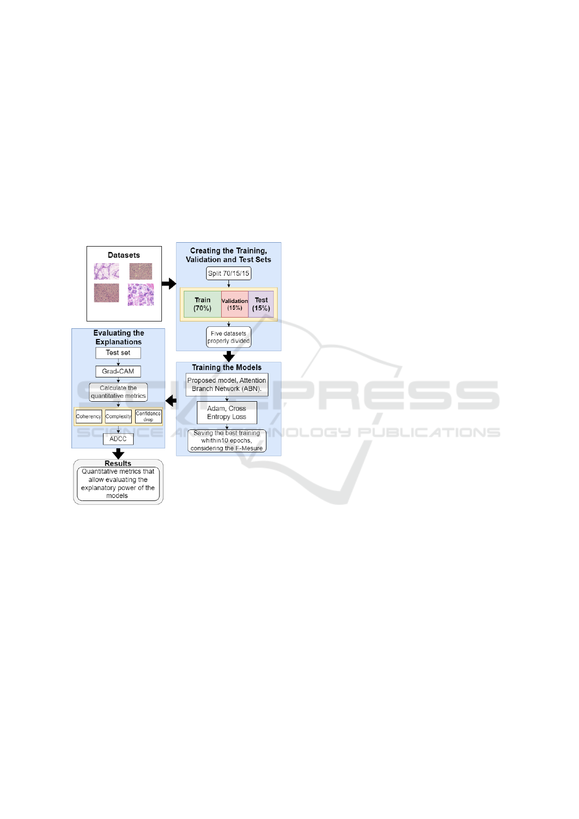
datasets of histological images, through the hold-out

strategy (Comet, 2023), considering a 70/15/15 split.

The second step consisted of training the ABN model

and the proposed model on each of the previously di-

vided datasets, using the F-measure as the metric for

selecting the best training among the epochs. Finally,

the models trained in the previous step were used to

obtain the activation maps of the images present in

the test split of each dataset, using the Grad-CAM

technique, so that all the quantitative metrics were

calculated to assess the explanatory capacity of each

model. An overview of the proposal is shown in Fig-

ure 1.

Figure 1: Proposed methodology to evaluate the explana-

tory capacity of the proposed architecture.

2.1 Proposed Architecture

To develop the architecture proposed in this work,

the approaches presented by (Fukui et al., 2019) and

(Sch

ottl, 2022) were considered. The proposed model

used two backbones, the ResNet-50 (He et al., 2016)

and DenseNet-201(Huang et al., 2017) networks.

These architectures were chosen because of the rele-

vant results presented in (Fukui et al., 2019). The pro-

posed architecture considered three modules (feature

extractor, attention branch and perception branch).

In addition, the proposed architecture considers two

mechanisms (the attention mechanism and CAM fos-

tering) aimed at improving explanations. Figure 2

gives an overview of the proposed architecture, which

also shows the proposed modiﬁcations made to the

ABN model.

The proposed model considered a feature extrac-

tor module based on all residual (ResNet-50) or dense

blocks (DenseNet-201), excluding the last block in

both cases. It is important to note that the last block

was not considered in this case, as it is used to com-

pose the attention branch and the perception branch.

The main purpose was to extract feature maps g(X

)

from the input image X

, where these maps were then

provided as input to the attention branch and attention

mechanism.

The attention branch module received the feature

maps g(X

) obtained by the feature extractor so that

these maps were then processed by a series of con-

volutional layers. The composition of these convolu-

tional layers is the same as those present in the last

residual (ResNet-50) or dense block (DenseNet-201)

from the backbone model. The output provided by

these convolutional layers is presented in the format

K × w × h, where K is the number of feature maps, w

is the width and h is the height of each map. This data

was then processed by a block composed of a batch

normalization layer, a 1 ×1 × 1 convolution layer and

a ReLU activation. This conﬁguration allowed all K

maps to be aggregated into a single map. The map

was then normalized by a block composed of a batch

normalization layer, a 1 ×1 × 1 convolution layer and

a sigmoid activation. Finally, an M(X

) attention map

was created in order to be used in the attention mech-

anism and CAM fostering mechanism. It is important

to note that, unlike the original ABN model, our at-

tention branch does not have the classiﬁcation module

for the attention map. This modiﬁcation was made in

order to use the CAM fostering strategy when training

the model.

The use of attention mechanisms has become

an increasingly common practice in different com-

puter vision systems, especially for sequential mod-

els (Yang et al., 2016; You et al., 2016; Vaswani et al.,

2017). For the proposed model, the attention mecha-

nism follows the indications of (Fukui et al., 2019).

From a set of feature maps g(X

) and an attention

map M(X

), it was possible to use the attention map to

create new feature maps g

′

), whose important ar-

eas for the model’s ﬁnal classiﬁcation are reinforced.

Equation 1 indicates the association of the attention

map with the feature maps.

′

) = (g(X

) × M(X

)) + g(X

) (1)

The perception branch was the module responsi-

ble for providing the ﬁnal classiﬁcation (label). This

module received the g

′

) feature maps as input and

ICEIS 2024 - 26th International Conference on Enterprise Information Systems

458

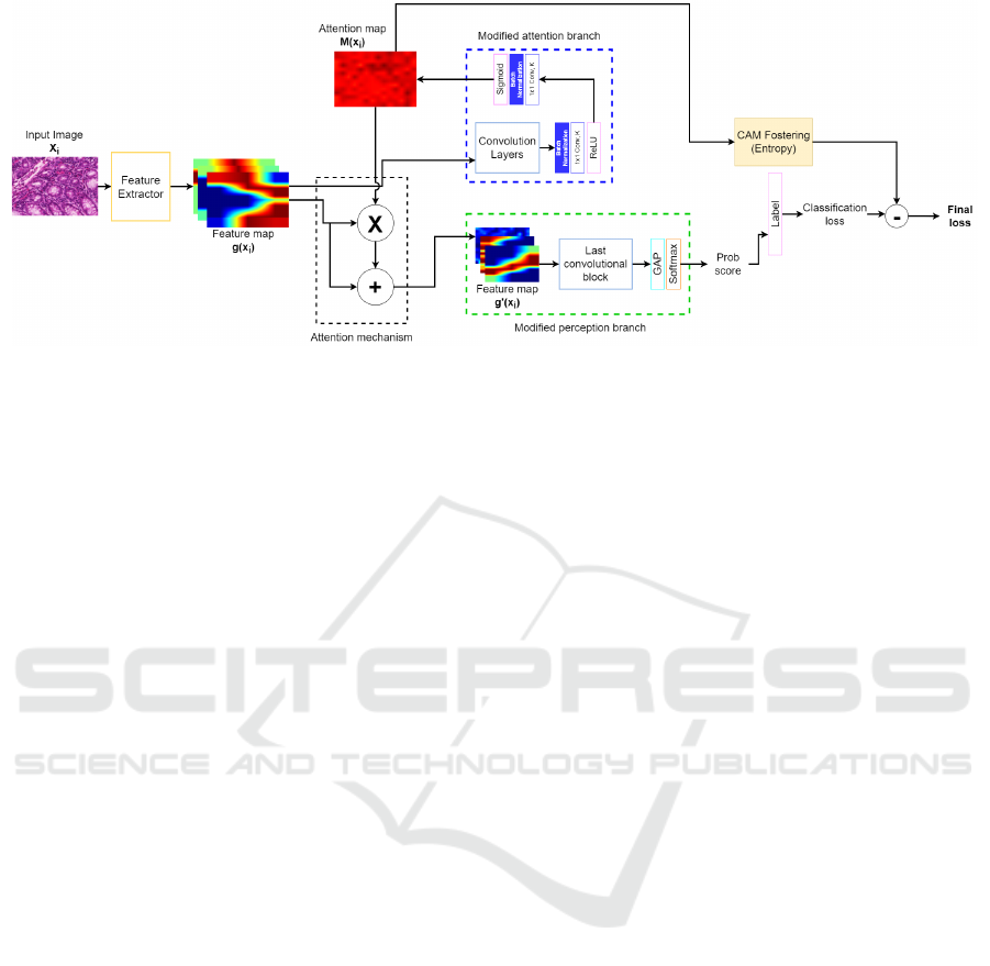
Figure 2: Overview of the proposed architecture, where the blue segmented rectangle shows the attention branch after the

proposed modiﬁcations, while the green segmented rectangle shows the perception branch after the modiﬁcations.

from the attention mechanism. The perception branch

was made up of convolutional layers that correspond

to the conﬁguration of the last residual (ResNet-50) or

dense block (ResNet-50) from the backbone model,

as well as a global average pooling layer (GAP) used

to provide the model’s ﬁnal classiﬁcation in associ-

ation with a softmax function. The choice to use the

GAP layer instead of the fully connected layer present

in the original ABN model followed the indications

presented by (Zhou et al., 2016). By using the GAP

layer to perform the model’s ﬁnal classiﬁcation, the

convolutional layers’ ability to locate objects in the

image is preserved, consequently improving the ar-

chitecture’s explanatory power.

The CAM fostering mechanism follows the de-

scription presented by (Sch

ottl, 2022), in which it is

possible to calculate the entropy value ce of an ac-

tivation map. The entropy computed from an activa-

tion map measures the variability of activations across

different regions or pixels in the map. A uniform map

with consistent activations yields low entropy, while a

varied map with diverse activations shows higher en-

tropy. Adding entropy as a term in the loss function

can serve as regularization, encouraging the model to

generate more diverse and information-rich activation

maps.

Thus, for the proposed model, the entropy factor

ce was calculated from the attention map M(X

) and

weighed by a regularization factor γ

equal to 10. The

chosen value for γ

followed the indications given by

(Sch

ottl, 2022). The weighed ce value was then sub-

tracted from the classiﬁcation loss l

measured by a

cross-entropy loss function (Mao et al., 2023), giving

the new loss value l

′

. Equation 2 shows how the ce

value is calculated, while Equation 3 shows how the

new loss value was calculated considering the CAM

fostering strategy.

ce(M(X

)) = −

∑

M(X

)

i j

− ln M(X

)

i j

(2)

′

= l

− γ

∗ ce(M(X

)), (3)

where i j represents the pixel’s index from the at-

tention map.

2.2 Dataset

This study used ﬁve datasets representing four differ-

ent types of histological tissues. For all ﬁve datasets,

the tissue samples were stained with hematoxylin and

eosin (H&E). The ﬁrst dataset (UCSB) is composed

of breast cancer images provided by the University

of California, Santa Barbara (Drelie Gelasca et al.,

2008). This dataset consists of 58 samples divided

into two classes: benign (32) and malignant (26).

The second dataset (CR) is composed of images of

colorectal tissues (Sirinukunwattana et al., 2017), to-

taling 165 samples divided between two classes: be-

nign (74) and malignant (91). To acquire the images,

histological areas were digitally photographed using

a Zeiss MIRAX MIDI Slide Scanner with a resolu-

tion scale of 0.620 µm, which is equivalent to a 20x

magniﬁcation.

The third dataset (NHL) was published by the Na-

tional Cancer Institute and the National Institute on

Ageing (Shamir et al., 2008), and consists of 173

samples of non-Hodgkin lymphoma divided into three

classes: MCL — mantle cell lymphoma (99); FL —

follicular lymphoma (62); and CLL— chronic lym-

phocyte leukemia (12). To obtain the images, a light

microscope Zeiss Axioscope with a 20x objective and

an AXio Cam MR5 digital camera were used. The

images obtained by this process were stored without

compression with a resolution of 1388 × 1040 pixels,

a 24-bit quantization ratio and the RGB color model;

Improving Explainability of the Attention Branch Network with CAM Fostering Techniques in the Context of Histological Images

459

Finally, the fourth and ﬁfth datasets were provided

by the Atlas of Gene Expression in Mouse Ageing

Project (AGEMAP) and are composed of liver tissue

images obtained from mice (AGEMAP, 2020). The

images were acquired by a Carl Zeiss Axiovert 200

microscope and 40x objective. The fourth dataset

(LG) consists of 265 liver tissue samples obtained

from male (150) and female (115) mice on a caloric

restriction diet. The ﬁfth dataset (LA) is composed

of 529 images divided into four classes, where each

class represents different age groups of female mice

on an ad libitum diet, the classes being: one (100);

six (115); 16 (162) and 24 (152) months old.

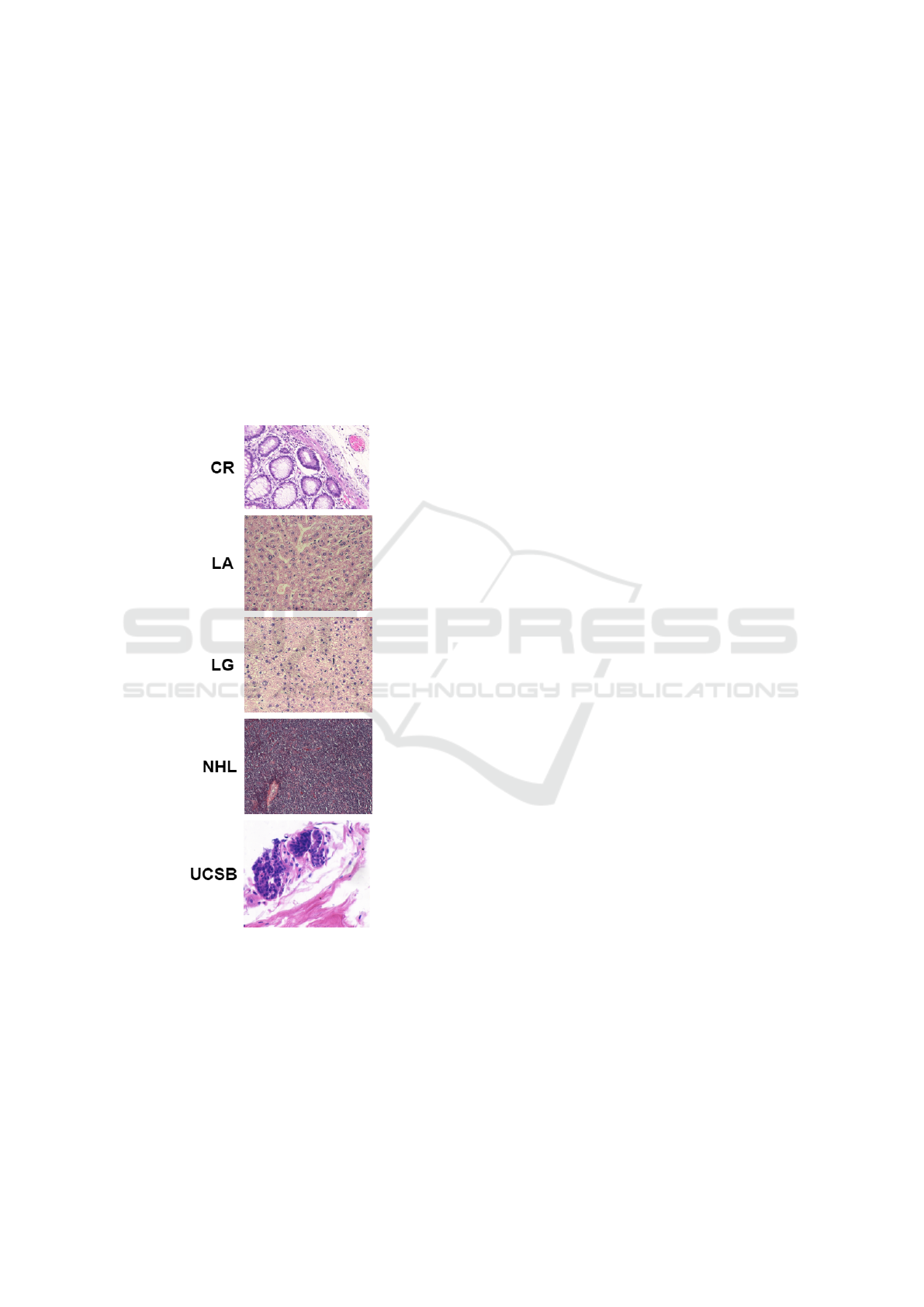
Figure 3 shows a sample from each dataset, while

Table 1 displays an overview of all datasets.

Figure 3: Examples of histological images from each

dataset: UCSB (Drelie Gelasca et al., 2008); CR (Sir-

inukunwattana et al., 2017); NHL (Shamir et al., 2008); LA

and LG (AGEMAP, 2020).

2.3 Step 1: Creating the Training,

Validation and Test Sets

To ensure consistent results in terms of the explana-

tory power of each compared model, the hold-out

strategy was applied to each dataset individually

(Comet, 2023). A 70/15/15 split was applied to each

dataset, whereby: 70% of the dataset was dedicated to

the training process, 15% to the validation stage, and

15% to the tests. It is worth noting that the images be-

longing to the split were randomly selected from the

original sets.

2.4 Step 2: Training the Models

For this step, the ABN models and the proposed

here were trained. In both cases, the ResNet-50 and

DenseNet-201 architectures were used as backbones,

so that a fair comparison could be made of the impact

of the modiﬁcations proposed by our methodology in

both cases. To speed up the training process and avoid

problems such as overﬁtting due to the small num-

ber of samples in some datasets, the transfer learning

strategy was applied (Zhuang et al., 2019). Therefore,

all models were pre-trained on the ImageNet image

database (Deng et al., 2009), so that it was possible to

ﬁne-tune the weights considering a small number of

epochs.

For training, a total of 10 epochs were chosen,

considering a learning rate of 0.0001 and a batch size

of 16. To update the weights, the Adam optimizer was

chosen given its rapid convergence, considering a re-

duced number of epochs (Kingma and Ba, 2014). It

is worth mentioning that all the weights in the model

were updated during the training step. The loss func-

tion chosen for training was the cross-entropy loss

(Mao et al., 2023). The loss value obtained loss value

was then used together with the CAM fostering strat-

egy to obtain a new loss value, which was used to

update the network weights during this step.

2.5 Step 3: Evaluating the Explanations

In this step, the quantitative metrics relating to the

quality of the Grad-CAM of each of the models

trained in step 2 were calculated. Thus, the set of

images belonging to the test split of each dataset pre-

viously deﬁned in step 1 was used to obtain the acti-

vation maps. The metrics used to assess the explana-

tory power of each model were proposed by (Poppi

et al., 2021) such as coherency, complexity, conﬁ-

dence drop and average DCC. The coherency metric

indicates that, given an image x referring to a class of

interest c, the activation map obtained by the image x

should not be altered when the activation map itself

is provided to the network. This property is presented

CAM

(x ⊙CAM

(x)) equal to CAM

(x). (4)

ICEIS 2024 - 26th International Conference on Enterprise Information Systems

460

Table 1: Overview of all ﬁve datasets.

Dataset Tissue type Classes Samples Resolution

UCSB Breast tumours 2 58 896 × 768

CR Colorectal tumours 2 165 From 567 × 430 to 775 × 522

NHL Non-Hodgkin lymphoma 3 173 From 86 × 65 to 1388 × 1040

LG Liver tissue 2 265 417 × 312

LA Liver Tissue 4 529 417 × 312

Therefore, to measure the extent to which an acti-

vation map respects this property, the Pearson Corre-

lation Coefﬁcient was calculated between two CAMs

considering Equation 5.

Coherency(x) =

Cov(CAM

(x ⊙CAM

(x)),CAM

(x))

σCAM

(x ⊙CAM

(x))σCAM

(x)

(5)

where Cov is the covariance between two maps

and σ indicates the standard deviation. It is worth

noting that as the Pearson Correlation Coefﬁcient is

deﬁned in the [-1, 1] interval, therefore, the values

obtained were subsequently normalized in the [0, 1]

interval to maintain the same scale as the other met-

rics. This metric takes on values closer to one when

the method is invariant to the input image.

The complexity metric was responsible for calcu-

lating the quantity of information presented in an acti-

vation map, since the more pixels an explanation has,

the more complex it is, making this explanation not so

signiﬁcant. Thus, adopting the L

norm as a proxy, it

was possible to calculate complexity using Equation

Complexity(x) = ∥CAM

(x)∥

(6)

Therefore, the lower the number of pixels as-

signed to a given explanation, the lower the complex-

ity value, this value being limited to the interval [0,

1].

The conﬁdence drop was a metric that indicated

the loss of conﬁdence in a model when only the acti-

vation map was provided as input instead of the full

image. This metric was deﬁned by Equation 7

Drop(x) = max(0,y

− o

)/y

, (7)

Where y

is the class score considering the com-

plete image, and o

is the class score considering the

activation map of the complete image. This metric

was deﬁned in the interval [0, 1], where the closer it

is to zero, the lower the model’s loss of conﬁdence.

Finally, considering all the metrics described

above, the Average DCC (ADCC) was calculated as

the harmonic mean between all the metrics, as deﬁned

by Equation 8.

ADCC(x) = 3



Coherency(x)

1 −Complexity(x)

1 − Drop(x)



−1

(8)

In this way, it was possible to assess the overall

quality of the explanations generated by the models

tested in this study using a single metric.

3 RESULTS

The methodology developed in this work was applied

to evaluate the explanatory power of the proposed

model concerning other models in the literature, con-

sidering the context of histological images. Thus, the

evaluation process was deﬁned via the quantitative

metrics coherency (COH), complexity (COM), conﬁ-

dence drop (CD) and Average DCC (ADCC). Tables 2

and 3 show the results obtained in the ﬁrst experiment,

considering the proposed model using the ResNet-50

and DenseNet-201 networks as backbones, respec-

tively.

Table 2: Percentage values for coherency (COH), com-

plexity (COM), conﬁdence drop (CD) and ADCC for the

proposed model (ResNet-50, ABN, CAM fostering, GAP),

considering all datasets.

Dataset COH↑ COM↓ CD↓ ADCC↑

LG 31.66 0.24 35.01 47.35

CR 31.82 0.13 12.00 54.32

NHL 25.13 0.07 62.50 35.32

UCSB 32.47 0.11 11.11 55.24

LA 20.82 0.24 77.22 26.35

Mean 28.38 0.16 39.57 43.72

Considering the results presented in Table 2, the

proposed model via the ResNet-50 network as a back-

bone showed the best results among all the experi-

ments. For the CR and UCSB datasets, the proposed

approach was able to achieve an ADCC index equal to

54.32% and 55.24% respectively, contributing to the

average of 43.72% achieved in this metric. This result

indicates that the model has an important explanatory

capability in the context of histological images. It is

Improving Explainability of the Attention Branch Network with CAM Fostering Techniques in the Context of Histological Images

461

Table 3: Percentage values for coherency (COH), complex-

ity (COM), conﬁdence drop (CD) and ADCC for the pro-

posed model (DenseNet-201, ABN, CAM fostering, GAP),

considering all datasets.

Dataset COH↑ COM↓ CD↓ ADCC↑

LG 28.44 0.23 52.40 24.96

CR 33.96 0.13 14.94 57.58

NHL 38.70 0.07 60.07 37.81

UCSB 32.92 0.11 15.95 56.02

LA 38.17 0.24 71.07 27.17

Mean 34.44 0.16 42.89 40.71

also relevant to highlight the coherence indices ob-

tained by this model, where it was observed that the

proposed approach was able to reach a value higher

than 30% in three of the ﬁve datasets, totaling an av-

erage of 28.38%. This indicates that this model has a

better ability to generate more concise explanations.

For the results obtained by the proposed model

using the DenseNet-201 network as a backbone, an

average ADCC metric of 40.71% was observed, es-

pecially for the CR dataset, where the conﬁguration

used in this test was able to achieve an ADCC value

of 57.58% which is the highest metric obtained in this

work. It is also important to note that this conﬁgu-

ration had the highest average coherence index of all

the models tested, with an average coherence value of

34.44%.

Taking into account the second experiment, the at-

tention branch network model (ABN) was evaluated

in the same way using the ResNet-50 and DenseNet-

201 architectures. Tables 4 and 5 show the results

obtained for each backbone, respectively.

Table 4: Percentage values for coherency (COH), complex-

ity (COM), conﬁdence drop (CD) and ADCC for the ABN

model (ResNet-50), considering all datasets.

Dataset COH↑ COM↓ CD↓ ADCC↑

LG 30.05 0.24 19.72 52.55

CR 26.36 0.13 4.75 50.13

NHL 23.57 0.07 54.84 27.84

UCSB 26.70 0.11 8.39 50.37

LA 15.82 0.24 75.34 16.94

Mean 24.50 0.16 32.60 39.56

Table 5: Percentage values for coherency (COH), complex-

ity (COM), conﬁdence drop (CD) and ADCC for the ABN

Model (DenseNet-201), considering all datasets.

Dataset COH↑ COM↓ CD↓ ADCC↑

LG 21.40 0.23 47.74 7.71

CR 32.66 0.13 29.84 54.08

NHL 24.43 0.07 60.51 19.10

UCSB 13.65 0.06 11.46 25.08

LA 31.21 0.24 74.48 23.24

Mean 24.67 0.15 44.81 25.84

For the results obtained by the ABN model us-

ing the ResNet-50 as a backbone, it was observed

that in three of the ﬁve datasets the ADCC metric

was greater than 50%, totaling an average ADCC of

39.56%. This result is 4.16% lower in relation to the

proposed model using the same backbone. It is also

important to highlight the conﬁdence drop index ob-

tained by the architecture in the CR dataset, where

a total of 4.75% was observed, the lowest value ob-

tained in all the experiments in this study. Finally,

it is worth noting the value of the coherence index

obtained by the ABN model, in which an average in-

dex of 24.50% was observed, this result being 3.88%

lower compared to the proposed model. These data

indicate that the model was unable to generate expla-

nations that showed more restricted areas in the im-

age.

As for the results presented by the ABN model

using the DesNet-201 network as a backbone, low

ADCC indices were observed for each of the ﬁve

datasets, totaling an average ADCC of 25.84%. This

result is 14.87% lower than the proposed model us-

ing the same backbone. It is also worth noting that

the average coherence value obtained by this model

was 24.67%, which is 9.77% lower than the model

proposed in this work. These results prove the effec-

tiveness of the modiﬁcations proposed in this study

in terms of increasing the explanatory power of the

models.

Finally, Figures 4 and 5 show some samples of

explanations obtained by the proposed model and the

ABN model, using the ResNet-50 and DenseNet-201

networks as backbones, respectively. These images

show the impact of the coherence metric on the ex-

planations generated by each model, where the ex-

planations are expected to have smaller areas that are

important for the ﬁnal classiﬁcation.

From the samples of explanations shown in ﬁg-

ures 4 and 5, it could be seen that the proposed model

was able to provide more concise explanations com-

pared to the ABN model using the same backbones,

a fact that is directly related to the coherence metrics

obtained by each model. Therefore, it is possible to

observe that the application of the proposed method-

ology was able to generate better explanations in the

context of histological image analysis.

4 CONCLUSIONS

In this work, a proposed model was deﬁned to

improve the attention branch network architecture

through the use of the CAM fostering strategy. The

proposal was tested to increase the explanatory power

ICEIS 2024 - 26th International Conference on Enterprise Information Systems

462

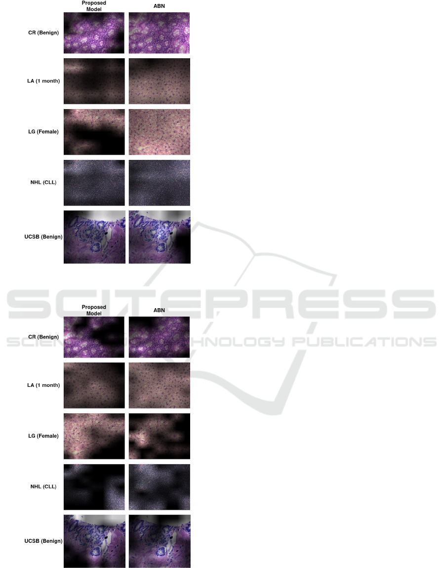
Figure 4: Explanations obtained with the Grad-CAM tech-

nique, considering the proposed model and the ABN model,

using the ResNet-50 as the backbone.

Figure 5: Explanations obtained with the Grad-CAM tech-

nique, considering the proposed model and the ABN model,

using the DenseNet-201 as the backbone.

of the model in the context of histological images.

Thus, a pipeline was developed to train the models,

as well as allow fair comparisons between the expla-

nations generated by the proposed approach and the

ABN model. In this pipeline, quantitative metrics

were used to assess the quality of the explanations

generated by each model.

The proposed model using the ResNet-50 network

as a backbone obtained the highest average ADCC

when compared to the other conﬁgurations tested

(43.3%), indicating an improvement of 4.16% when

compared to the ABN model using the same back-

bone. The model proposed using the DenseNet-201

network as a backbone showed a signiﬁcant improve-

ment in its explanatory power, reaching an average

ADCC of 40.71%. This shows that the proposed

model explanatory power was increased by 14.87%

when compared to the ABN model using the same

backbone. In addition, this conﬁguration provided the

best coherence metric in the study totaling an average

of 34.44%, which indicates that this model is capable

of creating explanations that emphasize only the most

important regions of the image. These results prove

that the modiﬁcations proposed in this work were able

to improve the explanatory power of the models, and

are important contributions to the development of re-

liable CAD systems.

For future work, we intend to investigate the im-

pact of the modiﬁcations using other models as back-

bones, as well as adapting the explanation evaluation

pipeline to support explanations generated by vision

transformer models.

ACKNOWLEDGEMENTS

This research was funded in part by the: Coordenac¸

de Aperfeic¸oamento de Pessoal de N

ıvel Superior

- Brasil (CAPES) – Finance Code 001; National

Council for Scientiﬁc and Technological Develop-

ment CNPq (#313643/2021-0 and #311404/2021-9);

the State of Minas Gerais Research Foundation -

FAPEMIG (Grant #APQ-00578-18); S

ao Paulo Re-

search Foundation - FAPESP (Grant #2022/03020-1);

WZTECH NETWORKS, S

ao Jos

e do Rio Preto, S

Paulo.

REFERENCES

AGEMAP, N. I. o. A. (2020). The atlas of gene expression

in mouse aging project. AGEMAP. https://ome.grc.ni

a.nih.gov/iicbu2008/agemap/index.html.

Comet (2023). Understanding hold-out methods for training

Improving Explainability of the Attention Branch Network with CAM Fostering Techniques in the Context of Histological Images

463

machine learning models. Comet. https://www.comet.

com/site/blog/understanding-hold-out-methods-for-t

raining-machine-learning-models.

Deng, J., Dong, W., Socher, R., Li, L.-J., Li, K., and Fei-

Fei, L. (2009). Imagenet: A large-scale hierarchical

image database. In 2009 IEEE conference on com-

puter vision and pattern recognition, pages 248–255.

Ieee.

Drelie Gelasca, E., Byun, J., Obara, B., and Manjunath, B.

(2008). Evaluation and benchmark for biological im-

age segmentation. In 2008 15th IEEE International

Conference on Image Processing, pages 1816–1819.

Fischer, A. H., Jacobson, K. A., Rose, J., and Zeller, R.

(2008). Hematoxylin and eosin staining of tissue and

cell sections. CSH Protoc, 2008:db.prot4986.

Fukui, H., Hirakawa, T., Yamashita, T., and Fujiyoshi, H.

(2019). Attention branch network: Learning of at-

tention mechanism for visual explanation. In 2019

IEEE/CVF Conference on Computer Vision and Pat-

tern Recognition (CVPR), pages 10697–10706.

Gurina, T. S. and Simms, L. (2023). Histology, Staining.

StatPearls Publishing.

He, K., Zhang, X., Ren, S., and Sun, J. (2016). Deep resid-

ual learning for image recognition. In 2016 IEEE Con-

ference on Computer Vision and Pattern Recognition

(CVPR), pages 770–778.

Huang, G., Liu, Z., Maaten, L. V. D., and Weinberger, K. Q.

(2017). Densely connected convolutional networks.

In 2017 IEEE Conference on Computer Vision and

Pattern Recognition (CVPR), pages 2261–2269, Los

Alamitos, CA, USA. IEEE Computer Society.

ohn, J., Krieghoff-Henning, E., Jutzi, T. B., von Kalle,

C., Utikal, J. S., Meier, F., Gellrich, F. F., Hobels-

berger, S., Hauschild, A., Schlager, J. G., French, L.,

Heinzerling, L., Schlaak, M., Ghoreschi, K., Hilke,

F. J., Poch, G., Kutzner, H., Heppt, M. V., Haferkamp,

S., Sondermann, W., Schadendorf, D., Schilling, B.,

Goebeler, M., Hekler, A., Fr

ohling, S., Lipka, D. B.,

Kather, J. N., Krahl, D., Ferrara, G., Haggenm

uller,

S., and Brinker, T. J. (2021). Combining cnn-based

histologic whole slide image analysis and patient data

to improve skin cancer classiﬁcation. European Jour-

nal of Cancer, 149:94–101.

Kingma, D. and Ba, J. (2014). Adam: A method for

stochastic optimization. International Conference on

Learning Representations.

Majumdar, S., Pramanik, P., and Sarkar, R. (2023). Gamma

function based ensemble of cnn models for breast can-

cer detection in histopathology images. Expert Sys-

tems with Applications, 213:119022.

Mao, A., Mohri, M., and Zhong, Y. (2023). Cross-entropy

loss functions: theoretical analysis and applications.

In Proceedings of the 40th International Conference

on Machine Learning, ICML’23. JMLR.org.

Miotto, R., Wang, F., Wang, S., Jiang, X., and Dudley, J. T.

(2017). Deep learning for healthcare: review, oppor-

tunities and challenges. Brieﬁngs in Bioinformatics,

19(6):1236–1246.

Poppi, S., Cornia, M., Baraldi, L., and Cucchiara, R. (2021).

Revisiting the evaluation of class activation mapping

for explainability: A novel metric and experimental

analysis. In 2021 IEEE/CVF Conference on Computer

Vision and Pattern Recognition Workshops (CVPRW),

pages 2299–2304.

Sch

ottl, A. (2022). Improving the interpretability of grad-

cams in deep classiﬁcation networks. Procedia Com-

puter Science, 200:620–628. 3rd International Con-

ference on Industry 4.0 and Smart Manufacturing.

Selvaraju, R. R., Cogswell, M., Das, A., Vedantam, R.,

Parikh, D., and Batra, D. (2019). Grad-CAM: Visual

explanations from deep networks via gradient-based

localization. International Journal of Computer Vi-

sion, 128(2):336–359.

Shamir, L., Orlov, N., Mark Eckley, D., Macura, T. J., and

Goldberg, I. G. (2008). Iicbu 2008: a proposed bench-

mark suite for biological image analysis. Medical

& Biological Engineering & Computing, 46(9):943–

947.

Shihabuddin, A. R. and K., S. B. (2023). Multi cnn

based automatic detection of mitotic nuclei in breast

histopathological images. Computers in Biology and

Medicine, 158:106815.

Sirinukunwattana, K., Pluim, J. P., Chen, H., Qi, X., Heng,

P.-A., Guo, Y. B., Wang, L. Y., Matuszewski, B. J.,

Bruni, E., Sanchez, U., B

ohm, A., Ronneberger, O.,

Cheikh, B. B., Racoceanu, D., Kainz, P., Pfeiffer,

M., Urschler, M., Snead, D. R., and Rajpoot, N. M.

(2017). Gland segmentation in colon histology im-

ages: The glas challenge contest. Medical Image

Analysis, 35:489–502.

Vaswani, A., Shazeer, N., Parmar, N., Uszkoreit, J., Jones,

L., Gomez, A. N., Kaiser, L. u., and Polosukhin,

I. (2017). Attention is all you need. In Guyon,

I., Luxburg, U. V., Bengio, S., Wallach, H., Fer-

gus, R., Vishwanathan, S., and Garnett, R., editors,

Advances in Neural Information Processing Systems,

volume 30. Curran Associates, Inc.

Xu, F., Uszkoreit, H., Du, Y., Fan, W., Zhao, D., and Zhu,

J. (2019). Explainable ai: A brief survey on history,

research areas, approaches and challenges. In Tang,

J., Kan, M.-Y., Zhao, D., Li, S., and Zan, H., edi-

tors, Natural Language Processing and Chinese Com-

puting, pages 563–574, Cham. Springer International

Publishing.

Yang, Z., He, X., Gao, J., Deng, L., and Smola, A. (2016).

Stacked attention networks for image question an-

swering. In 2016 IEEE Conference on Computer Vi-

sion and Pattern Recognition (CVPR), pages 21–29.

You, Q., Jin, H., Wang, Z., Fang, C., and Luo, J. (2016). Im-

age captioning with semantic attention. In 2016 IEEE

Conference on Computer Vision and Pattern Recog-

nition (CVPR), pages 4651–4659, Los Alamitos, CA,

USA. IEEE Computer Society.

Zhou, B., Khosla, A., Lapedriza, A., Oliva, A., and Tor-

ralba, A. (2016). Learning deep features for discrimi-

native localization. In 2016 IEEE Conference on Com-

puter Vision and Pattern Recognition (CVPR), pages

2921–2929, Los Alamitos, CA, USA. IEEE Computer

Society.

Zhuang, F., Qi, Z., Duan, K., Xi, D., Zhu, Y., Zhu, H.,

Xiong, H., and He, Q. (2019). A comprehensive sur-

vey on transfer learning. CoRR, abs/1911.02685.

ICEIS 2024 - 26th International Conference on Enterprise Information Systems

464