Stock Market Forecasting Using Machine Learning Models Through

Volatility-Driven Trading Strategies

Ivan Letteri

Department of Life, Health and Environmental Sciences, University of L’Aquila, Italy

Keywords:

Machine Learning, Statistical Analysis, Algorithmic Trading, K-Means++, Granger Causality Test.

Abstract:

The purpose of our research was to explore volatility-based trading strategies in ﬁnancial markets to leverage

market dynamics for capital gain. We sought to introduce a strategy that integrated statistical analysis with ma-

chine learning to predict stock market trends. Our method involved using the k-means++ clustering algorithm

to examine the mean volatility of the nine largest stocks in both the NYSE and Nasdaq markets. The clusters

formed the basis for understanding relationships among stocks based on their volatility patterns. We further

subjected the mid-volatility clustered dataset to the Granger Causality Test, which helped identify stocks with

strong predictive connections. These stocks were crucial in formulating our trading strategy, serving as trend

indicators for decisions on target stock trades. Our empirical approach included thorough backtesting and

performance analysis. Our ﬁndings demonstrated the effectiveness of our method in exploiting proﬁtable trad-

ing opportunities. This was achieved through predictive insights derived from volatility clusters and Granger

causality relationships among stocks. In conclusion, our research contributed to the ﬁeld of volatility-based

trading strategies by offering a methodology that combined a statistical approach with machine learning. This

enhanced the predictability of stock market trends.

1 INTRODUCTION

The ﬁeld of ﬁnance is witnessing a growing interest in

volatility-based trading, which capitalises on market

dynamics. Artiﬁcial Intelligence (AI) plays a crucial

role in this, providing robust tools for analysing and

leveraging market volatility. Speciﬁcally, AI’s abil-

ity to estimate mean volatility offers valuable insights

into the uncertainty and risk associated with speciﬁc

securities or the overall market (Letteri et al., 2022).

In our work, the key research questions include

examining the effectiveness of k-means++ clustering

in analyzing the mean volatility of major stocks, un-

derstanding relationships among stocks based on dis-

tinctive volatility patterns, and utilizing the Granger

Causality Test to assess predictive inﬂuences between

stocks. The study aims to formulate trading strategies

based on identiﬁed predictive connections, leveraging

inﬂuential stocks as trend indicators. Rigorous back-

testing and performance analysis validate the reliabil-

ity of the proposed volatility-driven trading strategy.

To answer the aforementioned research questions,

we created an AI trading strategy using k-means++

https://orcid.org/0000-0002-3843-386X

clustering of average volatility data (Arthur and Vas-

silvitskii, 2007) from nine major stock markets. Ini-

tially, we aim to identify distinct volatility patterns in

the market and group assets accordingly. We then uti-

lize the Granger Causality Test (GCT) (Kirchg

assner

and Wolters, 2007) to pinpoint stocks that signiﬁ-

cantly predict others in our analysis, establishing buy,

sell, or hold trading decisions.

In this study, we used the AITA framework (Let-

teri, 2023a) to rigorously analyse the historical per-

formance of the proposed strategy, employing multi-

ple performance metrics to evaluate its proﬁtability,

effectiveness, and resilience.

Previously, our focus on technical trading strate-

gies emphasised technical indicators (Letteri et al.,

2022),(Letteri et al., 2023), particularly for invest-

ment timing. We now explore Historical Volatility es-

timators as a dataset for identifying medium volatil-

ity and selecting stocks for the Granger Causality

Test asset cointegration approach (Engle and Granger,

1987).

This paper is organised as follows: Section 2

introduces foundational concepts within our AITA

framework, highlighting the Volatility Trading Sys-

tem (VolTS)(Letteri, 2023b) module and Aita Back-

Letteri, I.

Stock Market Forecasting Using Machine Learning Models Through Volatility-Driven Trading Strategies.

DOI: 10.5220/0012607200003717

Paper published under CC license (CC BY-NC-ND 4.0)

In Proceedings of the 6th International Conference on Finance, Economics, Management and IT Business (FEMIB 2024), pages 96-103

ISBN: 978-989-758-695-8; ISSN: 2184-5891

Testing (AitaBT). Section 3 outlines the methodol-

ogy within the VolTS module, which analyses securi-

ties’ volatility averages and establishes predictive re-

lationships. It then delves into the implementation of

the trading strategy and includes a thorough empirical

analysis of its performance and robustness. Section

4 presents practical ﬁndings achieved through back-

testing with the AitaBT module, followed by a dis-

cussion. Finally, Section 5 concludes the study by

summarising the effectiveness and applicability of the

proposed method.

2 BACKGROUND

2.1 Price Action

The price action (PA) inﬂuences Historical Volatility

(HV), and in turn, HV can provide insights into future

PA. When the PA exhibits strong price movements,

such as wide trading ranges, breakouts, or rapid di-

rectional changes, it tends to increase.

VolTS, a module within the AITA framework, ad-

heres to these principles. Low HV signiﬁes a pe-

riod of consolidation or low price volatility, indi-

cating a potential upcoming spike in volatility or a

shift in the PA. On the other side, high HV suggests

a higher probability of sharp market movements or

trend changes.

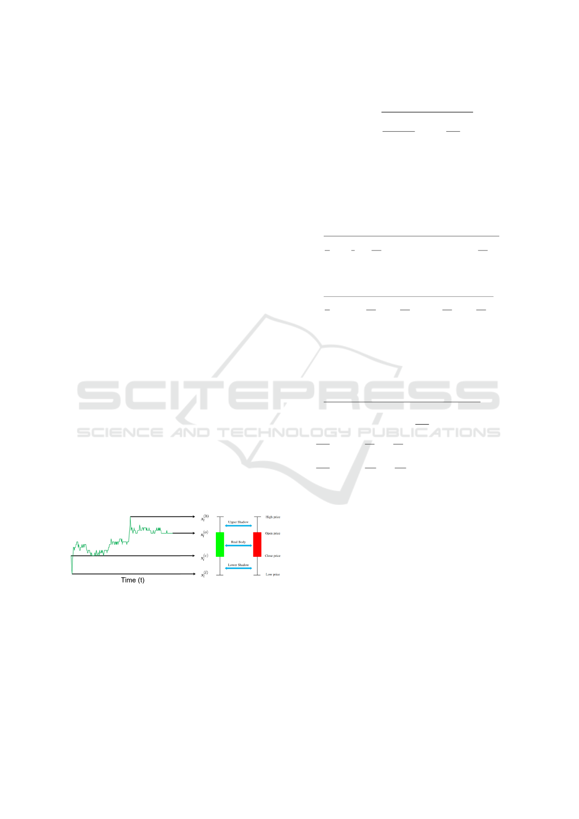
Within VolTS, the PA is encoded as OHLC, i.e.,

the open, high, low, and close prices of the assets,

as represented in the candlesticks charts (see ﬁg-

ure 1). For each timeframe t, the OHLC of an as-

set is represented as a 4-dimensional vector X

(o)

(h)

(l)

(c)

)

, where x

(l)

> 0, x

(l)

< x

(h)

and

(o)

(c)

∈ [x

(l)

(h)

Figure 1: Example of candlestick chart.

2.2 Historical Volatility Module

The construction of the dataset is designed to use the

following HV estimators:

- The Parkinson (PK) estimator incorporates the

stock’s daily high and low prices as follow:

PK =

4Nln(2)

∑

i=1

(h)

(l)

It is derived from the assumption that the true

volatility of the asset is proportional to the log-

arithm (ln) of the ratio of the high x

(h)

and low

(l)

prices of N observations.

- The Garman-Klass (GK) estimator as-

sumes that price movements are log-

normally distributed calculated as follows:

∑

i=1



(h)

(l)



−

∑

i=1

(2ln(2) − 1)



(c)

(o)



- The Rogers-Satchell (RS) estimator uses the range

of prices within a given time interval as a proxy

for the volatility of the asset as follows: RS =

∑

t=1



(h)

(c)





(h)

(o)



+ ln



(l)

(c)





(l)

(o)



RS assumes that the range of prices within the in-

terval is a good proxy for the volatility of the as-

set, additionally, the estimator may be sensitive to

outliers and extreme price movements.

- The Yang-Zhang (YZ) estimator

(Yang and Zhang, 2000) incorpo-

rates OHLC prices as follows: Y Z =

OvernightVol

+ kσ

OpenToCloseVol

+ (1 − k)σ

where k = 0.34/1.34 +

N+1

N−1

, σ

OpenToCloseVol

N−1

∑

i=1



(c)

(o)

− ln

(c)

(o)



, and σ

OvernightVol

N−1

∑

i=1



(o)

(c)

t−1

− ln

(o)

(c)

t−1



Empirical studies have demonstrated that the YZ

estimator exhibits notable performance across a

broad spectrum of scenarios, including those char-

acterised by jumps and non-normality in the data.

However, this estimator is not without its limita-

tions, and its effectiveness may be constrained in

certain contexts.

In this research, our attention is centred on mid-

volatility. This focus allows us to either close open

positions or refrain from entering a position when the

anticipated volatility coefﬁcient is high, thereby mit-

igating the risk of losses. On the other hand, if the

expected volatility is too low, it does not offer any po-

tential for gains.

2.3 Trading Strategies

Three distinct trading strategy classes are imple-

mented in AITA framework:

Stock Market Forecasting Using Machine Learning Models Through Volatility-Driven Trading Strategies

- Buy and Hold (B&H) strategy is used as a bench-

mark to compare the performance of the two

strategies below. It involves buying one single

share on the ﬁrst date of the period studied on the

market close and selling the share at the market

close on the last date as follows: V

= Q·P

, where

is the value of the investment at time t. Q is the

quantity of the asset purchased at time t = 0, and

is the price of the asset at time t with P

the

initial price.

- Trend Following (TF) strategy is one way to en-

gage in trend trading, where a trader initiates an

order in the direction of the breakout after the

price surpasses the resistance line as follows: let

the price at time t, and let MA denote the Mov-

ing Average of the asset price over a certain pe-

riod. If P

≥ MA

indicates an upward trend to

take a long position otherwise it is a downward

trend to take a short position.

- Mean Reversion (MR) strategy suggests that a se-

curity’s maximum and minimum prices are tem-

porary, and the security will eventually move to-

wards its mean as follows: let P

the price of the

asset at time t, and let µ and σ represent the mean

and standard deviation of the asset price, respec-

tively. The entry/exit conditions for a long/short

position are given by: P

< µ − k · σ and P

µ − k · σ, respectively where k is a constant rep-

resenting the number of standard deviations from

the mean at which the entry condition is triggered.

For the sake of brevity, in this study, the experiment

is focused on the trend-follow strategy and we com-

pare it with the B&H considered as a benchmark. It is

important to note that both trend-following and mean

reversion strategies, which are theoretically opposing

concepts, can be applied to the same stock without

conﬂicting with each other. Nonetheless, we ﬁnd it

beneﬁcial to apply the mean reversion strategy when

dealing with mid-volatility assets.

2.4 Backtesting Module

AitaBT module considers both proﬁt and risk metrics

as crucial factors in trading, in order to evaluate the

potential proﬁtability of investments and manage risk

exposure.

• (i) Drawdown (DD) is a measure of the peak-to-

trough decline in the value of a trading account

before a new peak is attained. DD is deﬁned as

follows: DD =

P−T

, where P is the highest value

or peak of the portfolio. T is the lowest value

or trough after the peak. Maximum Drawdown

(MDD) is the most signiﬁcant loss from peak to

trough during a speciﬁc period calculated as fol-

lows: MDD = max



−min

j:i≤ j≤N



, where P

the highest value or peak of the portfolio time i.

is the lowest value or trough after the peak up

to time j. N is the total number of data points.

• (ii) The Sortino ratio (SoR) is a risk-adjusted

proﬁt measure, which refers to the return per unit

of deviation as follows: SoR =

−R

, where R

the expected portfolio return, R

the risk-free rate

of return, and σ

denotes the downside deviation

of the portfolio returns.

• (iii) The Sharpe ratio (SR) is a variant of the risk-

adjusted proﬁt measure, which applies σ

as a risk

measure: SR =

−R

where σ

is the standard

deviation of the portfolio return.

• (iv) The Calmar ratio (CR) is another variant of

the risk-adjusted proﬁt measure, which applies

MDD as risk measure: CR =

−R

MDD

To check the goodness of trades, we mainly focused

on the Total Returns T R

(t) for each stock (k =

1,..., p) in the time interval (t = 1,...,n) with the price

P, deﬁned as follows:

T R

(t) =

(t +∆t) − P

(t)

Furthermore, we analyzed the standardized re-

turns r

= (T R

− µ

)/σ

, with (k = 1,..., p), where

is the standard deviation of T R

, e µ

denote the

average overtime for the studied period.

3 METHOD

3.1 Asset Collections

AITA automatically downloads the OHLC prices via

an internal Python library connected to an API, using

the MetaTrader5 (MT5)

directly associated with the

broker TickMill

. The data collected for this study

includes the OHLC prices of the stocks listed in Table

3.2 Anomalies Filtering

AITA framework starts to examine the price time

series of the assets to determine the time window

without considerable anomalies. The criterion im-

plemented is based on the anomaly score calculated

https://www.metatrader5.com/

https://tickmill.eu

FEMIB 2024 - 6th International Conference on Finance, Economics, Management and IT Business

Table 1: List of the main 9 stocks selected for the experi-

mentation.

Ticker Company Market

MSFT Microsoft Corporation Nasdaq

GOOGL Alphabet Inc. Nasdaq

MU Micron Technology, Inc. Nasdaq

NVDA NVIDIA Corporation NYSE

AMZN Amazon.com, Inc. NYSE

META Meta Platforms, Inc. NYSE

QCOM QUALCOMM Incorporated Nasdaq

IBM Int. Business Machines Corp. NYSE

INTC Intel Corporation NYSE

by a K-Nearest Neighbors (KNN) model (Wahid and

Chandra Sekhara Rao, 2020). One of the key ad-

vantages of KNN is its ability to handle non-linear

and complex relationships between data points (Let-

teri et al., 2021a)(Letteri et al., 2020a). The KNN

model is ﬁt to the time series data and the anomaly

score is calculated based on the distance between the

points and their k nearest neighbours.

The threshold (th) for detecting anomalies is then

determined based on the mean (µ) and standard devi-

ation (σ) of the anomaly scores. The criterion can be

expressed as follows: let x

be the value of the time se-

ries at time t, and k be the number of Nearest Neigh-

bours to use in the KNN model with the Euclidean

distance between x

and x

, where x

is the i

nearest

neighbour (NN) of x

. The anomaly score (as

) for x

is deﬁned as follow:

t,i

∑

− x

)

,∀i ∈ NN(x

,k).

The threshold th for detecting anomalies as fol-

lows: th = µ + 3 · σ. Data points with anomaly scores

greater than the threshold are considered to be anoma-

lies.

Figure 2 shows only one critical anomaly during

March 2020 (the global pandemic), so we decided to

use only the time window in the period after instead

of simply removing it, starting from 1st May 2020 to

1st May 2023.

3.3 Historical Volatility Dataset

The History Volatility Clustering process of our

approach determines the stocks with intermediate

volatility. First calculate the average of historical

volatility time series among the aforementioned es-

timators (see sect. 2.2). Next, the resulting volatil-

ity series are clusterized using the KMeans++ algo-

rithm with the Dynamic Time Warping (DTW) met-

ric (Niennattrakul and Ratanamahatana, 2007). DTW

is used to compare couples of time series that may

have different lengths and speeds of variation, which

makes it well-suited for this type of clustering. In

particular, we split into three clusters (K = 3) high,

middle, and low volatility. The centroids are selected

using the maximum DTW distance with respect to the

previous centroid.

Figure 3 shows the results displayed through a

plot of the time series belonging to the middle cluster

where we are focused on our strategy. It is worth not-

ing that, the main region is in the time window from

1st November 2022 to 1st May 2023. So, we use this

interval as the dataset, and then from the intermediate

cluster, the candidate assets selected are TSLA with

the highest, AMZN and META in the middle, with

QCOM and IBM with the lowest values, respectively.

3.4 Regression Analysis

AITA performs regression analysis to determine

whether one time series can predict another. Initially,

it uses linear regression to model how one variable

(independent variable) explains or predicts changes

in another variable (dependent variable) considering

F-statistic and Durbin-Watson statistics.

• F-statistic (F-stat) is used by VolTS to evaluate

the overall adequacy of the model by comparing

the full model with a null model (without any in-

dependent variables) by determining whether at

least one of the independent variables contributes

signiﬁcantly to explaining the variations in the de-

pendent variable.

• Durbin-Watson statistic calculated by VolTS de-

tects autocorrelation in the model residuals be-

cause it can inﬂuence the interpretation of the re-

sults. A value close to 2 indicates no autocorre-

lation, while values signiﬁcantly different from 2

suggest the presence of autocorrelation.

3.5 Cointegration and Causality

Cointegration refers to the long-term equilibrium re-

lationship between two or more time series. If two

time series are cointegrated, it means there exists a

stable linear combination between them, even if the

individual series may be non-stationary.

In the context of volatility-based trading, the

VolTS module performs the GCT to examine the re-

lationship between the lagged volatility of one asset

and the future volatility of another asset by applying

the following steps:

• Step 1. Signiﬁcant Granger causality: Let X

and Y be the pair stocks time series volatility to

check, where X represents the potential causal

Stock Market Forecasting Using Machine Learning Models Through Volatility-Driven Trading Strategies

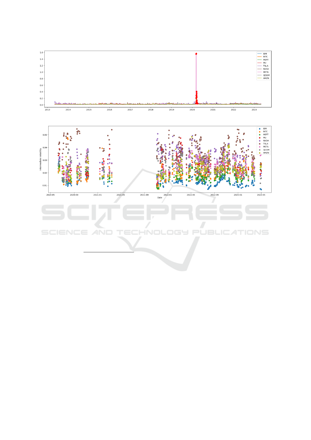
Figure 2: Red dots highlight the anomalies detected in the interval analyzed from 2020/05/01 to 2023/05/01.

Figure 3: Kmeans++ clusters with k = 3 of the Historical Volatility estimators dataset, from 1st May 2020 to 1st May 2023.

variable and Y represents the potential effect vari-

able. The null hypothesis (H0) states that X does

not Granger cause Y , while the alternative hypoth-

esis (H1) states that X does Granger cause Y . The

F-test is deﬁned as follows:

F − test =

[(RSS

Y (t)

− RSS

Y X

(t)

)/p]

[(RSS

Y X

(t)

)/(n − p − k)]

where RSS is the Residual Sum of

Squares for the two AutoRegressive mod-

els: Y(t) = c

+ β

∗ Y (t − 1) + β

∗

Y (t − 2) + · · · + β

∗ Y (t − p) + ε

Y (t)

, and

X : Y (t) = c

Y X

+ β

Y X

∗ X(t − 1) + β

Y X

∗ X(t −

2) + · · · + β

Y X

∗ X(t − p) + ε

Y X (t)

, with p the lag

order, n the number of observations, and k the

number of parameters in the models.

• Step 2. F-statistic comparison with the critical

value from the F-distribution where the signif-

icance level has α = 0.05. If the F-statistic is

greater than the critical value, reject the null hy-

pothesis (H0) and conclude that X Granger causes

Y with statistical signiﬁcance. If the F-statistic is

not greater than the critical value, fail to reject the

null hypothesis (H0) and conclude that there is

no signiﬁcant Granger causality between X and Y .

• Step 3. Direction of causality: If the volatility of

Stock X Granger causes the volatility of Stock Y ,

it suggests that changes in Stock X’s volatility can

be used to predict changes in Stock Y’s volatility.

3.6 The Algorithm

• Regression Step: For each pair of time series

), where i ̸= j, we construct a linear regres-

sion model:

= β

0,i j

+ β

1,i j

+ ε

i j

where β

0,i j

is the intercept, β

1,i j

is the regression

coefﬁcient, and ε

i j

is the error term. We calculate

the F-statistic and the Durbin-Watson statistic to

evaluate the overall adequacy of the model and de-

tect autocorrelation in the residuals, respectively.

• GCT Step: For each pair of time series (X

we perform the Granger causality test. The

model for the Granger test can be expressed as

(t) = α

i j

∑

k=1

k,i j

(t − k) +

∑

k=1

k,i j

(t −

k) + ε

i j

(t), where X

(t) is the current value of X

(t − k) and Y

(t − k) are the lagged values of X

and Y

, respectively, and ε

i j

(t) is the error term. If

the coefﬁcients γ

k,i j

are statistically different from

zero, we reject the null hypothesis and conclude

that Y

Granger causes X

FEMIB 2024 - 6th International Conference on Finance, Economics, Management and IT Business

100

4 RESULTS AND DISCUSSIONS

4.1 The Experiment

Figure 4: Co-integration via GCT.

The VolTS algorithm iterates the daily lags in a range

from 2 to 30 days to determine the best result. In this

experiment, the best result is achieved with lags=5,

where ’best’ is considered when there is direction co-

herency among the stocks with the maximum cardi-

nality of the set of stocks. In other words, the GCT

direction does not generate the acyclic graph in the

connection among the highest number of nodes, as

shown in ﬁgure 5.

In ﬁgure 7, we can see how the GCT suggests buy-

ing QCOM when META has a positive trend and vice

versa, the same thing with MU. Furthermore, when

AMZN price increases, it is time to buy META and

so on.

Figure 5: The best Acyclic Graph of the co-integration.

Figure 6 shows the scatter plot to visualise

whether there are patterns in the residuals that suggest

autocorrelation and to assess the overall adequacy of a

regression model. We can see how the stocks META,

QCOM, and AMZN conﬁrmed their autocorrelation.

The experiment results indicate that the volatility-

based trading strategy has performed well during the

tested period from 8th April 2023 to 1st June 2023.

The strategy resulted in a total gain of 231.77$ in 40

days of market opening, starting with an initial budget

of 1000$ per stock. The exposure time of the posi-

tions being open was quite high at 88.89% for all the

stocks, indicating active trading and frequent changes

in the portfolio.

Tab. 2 contains further details about the perfor-

mance metrics of the strategy and shows how the to-

tal amount in the portfolio is increased to 3231.77$

(7.725%), which is a positive sign of proﬁtable trad-

ing, also considering the ﬁxed commission of 9$ per

trade. Notice that, the managing of the budget is set

in compounded mode, so the full amount is reused for

each trade.

4.2 The Backtesting

The analysis of individual stocks’ performance is pre-

sented in ﬁgure 8 about META co-integration. The

trades of META bought following the AMZN trend

resulted in a Proﬁt and Loss (PnL) of 1.281%, with

a return of 9.721%. This return outperforms the

B&H strategy, which would have yielded a return of

6.684%.

Figure 9 shows the trades of QCOM bought fol-

lowing the META trend showed a PnL of 2.774%,

with a return of 12.866% compared to the B&H re-

turn of 9.235%. Furthermore, the trades of QCOM

bought following the MU trend resulted in a PnL of

1.562%, with a return of 6.302% as opposed to the

B&H return of 3.969%.

We compare, our backtesting trades to the opti-

mal portfolio derived against 10000 possible portfo-

lios constructed, in the same testing period, using the

Markowitz Efﬁcient Frontier (MEF), with the same

3000$ of budget and the constraint of 1000$ invested

in META and 2 × 1000$ in QCOM. MEF identiﬁes

the best portfolio with the highest T R of 3164.94$

when the volatility, measured with the standard de-

viation (72.41), is in the average. This conﬁrms our

idea to exploit the mid-volatility and highlights that

our trading approach wins with a T R of 3231.77$, so

2.23% more than the optimal portfolio.

5 CONCLUSION

In this work, we propose an effective method to han-

dle volatility in trading strategy and combine causal-

ity by the Historical Volatility Granger Causality Test

implemented in the AITA framework with the mod-

ule VolTS. The innovation of our system lies in select-

ing moderately volatile assets using Historical Volatil-

ity Estimators on market data and determining the

most proﬁtable stock pairings using K-means++ com-

bined with a statistical method to choose the predic-

tive property of our approach.

Stock Market Forecasting Using Machine Learning Models Through Volatility-Driven Trading Strategies

101

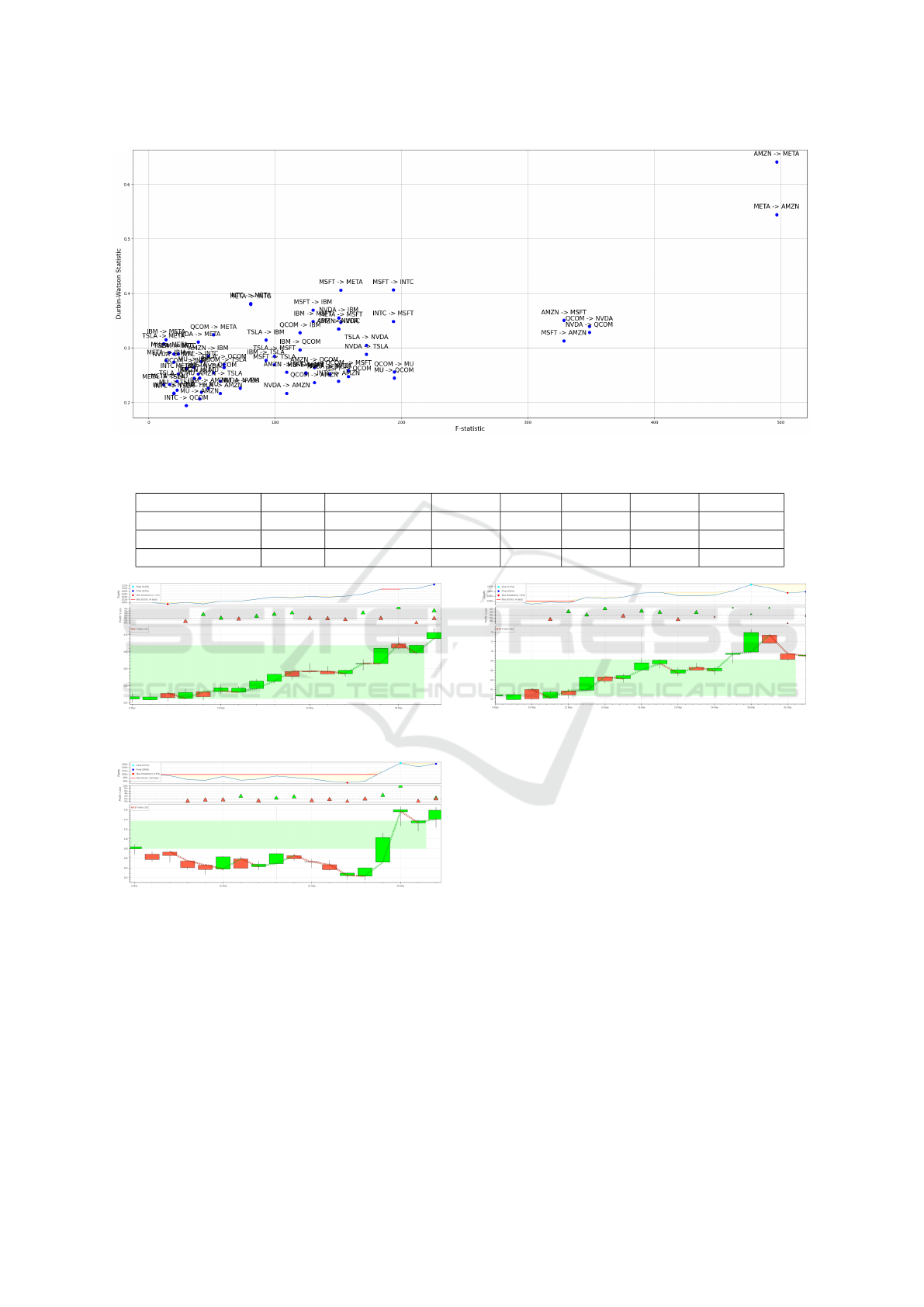
Figure 6: F-Statistic for regression model evaluation and Durbin-Watson statistics for autocorrelation in residuals.

Table 2: Results of the backtesting in the experiment.

Stock Trades Win rate (%) TR ($) SR SoR CR MDD (%)

AMZN ->META 16 37.5 1045.01 1.1784 4.6421 14.264 1.77

META ->QCOM 16 43.75 1110.11 3.8511 44.4613 248.342 -1.33

MU ->QCOM 16 56.25 1076.65 1.2130 6.3624 23.687 -7.65

Figure 7: Co-integration AMZN to META without spurious

correlation.

Figure 8: Co-integration META to QCOM without spurious

correlation.

Our future research areas include improving text

data handling techniques through dataset optimiza-

tion approaches (Letteri et al., 2020b),(Letteri et al.,

2021b) and incorporating domain expert knowledge

to enhance the model’s understanding of price and

volume data. Furthermore, we will expose the AITA

framework’s API as a secure service to thwart bot-

net attacks using Deep Learning models (Letteri et al.,

2019b)(Letteri et al., 2019a). To enhance resilience,

we plan to create a Multi-agent System which fea-

Figure 9: Co-integration MU to QCOM without spurious

correlation.

tures transparent Ethical Agents for customer service

(Dyoub et al., 2020) or combines logic constraint and

DRL (Gasperis et al., 2023). We will evaluate dia-

logues (Dyoub et al., 2021) with guidance from an

ethical teacher (Dyoub et al., 2022), also in other con-

texts like technology-enhanced learning (Angelone

et al., 2023).

REFERENCES

Angelone, A., Letteri, I., and Vittorini, P. (2023). First eval-

uation of an adaptive tool supporting formative assess-

ment in data science courses. In Methodologies and

Intelligent Systems for Technology Enhanced Learn-

ing, 13th International Conference, MIS4TEL 2023,

Guimaraes, Portugal, 12-14 July 2023, volume 764 of

Lecture Notes in Networks and Systems, pages 144–

151. Springer.

Arthur, D. and Vassilvitskii, S. (2007). K-means++: The

advantages of careful seeding. In Proceedings of the

FEMIB 2024 - 6th International Conference on Finance, Economics, Management and IT Business

102

Eighteenth Annual ACM-SIAM Symposium on Dis-

crete Algorithms, SODA ’07, page 1027–1035, USA.

Society for Industrial and Applied Mathematics.

Dyoub, A., Costantini, S., and Letteri, I. (2022). Care robots

learning rules of ethical behavior under the supervi-

sion of an ethical teacher (short paper). In Joint Pro-

ceedings of the 1st International Workshop on HYbrid

Models for Coupling Deductive and Inductive ReA-

soning (HYDRA 2022) and the 29th RCRA Workshop

on Experimental Evaluation of Algorithms for Solv-

ing Problems with Combinatorial Explosion (RCRA

2022) co-located with the 16th International Confer-

ence on Logic Programming and Non-monotonic Rea-

soning (LPNMR 2022), Genova Nervi, Italy, Septem-

ber 5, 2022, volume 3281 of CEUR Workshop Pro-

ceedings, pages 1–8. CEUR-WS.org.

Dyoub, A., Costantini, S., Letteri, I., and Lisi, F. A.

(2021). A logic-based multi-agent system for ethi-

cal monitoring and evaluation of dialogues. In Pro-

ceedings 37th International Conference on Logic Pro-

gramming (Technical Communications), ICLP Tech-

nical Communications 2021, Porto (virtual event), 20-

27th September 2021, volume 345 of EPTCS, pages

182–188.

Dyoub, A., Costantini, S., Lisi, F. A., and Letteri, I. (2020).

Logic-based machine learning for transparent ethical

agents. In Proceedings of the 35th Italian Conference

on Computational Logic - CILC 2020, Rende, Italy,

October 13-15, 2020, volume 2710 of CEUR Work-

shop Proceedings, pages 169–183. CEUR-WS.org.

Engle, R. F. and Granger, C. W. J. (1987). Co-integration

and error correction: Representation, estimation, and

testing. Econometrica, 55(2):251–276.

Gasperis, G. D., Costantini, S., Rafanelli, A., Migliarini,

P., Letteri, I., and Dyoub, A. (2023). Exten-

sion of constraint-procedural logic-generated environ-

ments for deep q-learning agent training and bench-

marking. J. Log. Comput., 33(8):1712–1733.

Kirchg

assner, G. and Wolters, J. (2007). Granger Causal-

ity, pages 93–123. Springer Berlin Heidelberg, Berlin,

Heidelberg.

Letteri, I. (2023a). AITA: A new framework for trading

forward testing with an artiﬁcial intelligence engine.

In Proceedings of the Italia Intelligenza Artiﬁciale -

Thematic Workshops co-located with the 3rd CINI Na-

tional Lab AIIS Conference on Artiﬁcial Intelligence

(Ital IA 2023), Pisa, Italy, May 29-30, 2023, volume

3486 of CEUR Workshop Proceedings, pages 506–

511. CEUR-WS.org.

Letteri, I. (2023b). Volts: A volatility-based trading system

to forecast stock markets trend using statistics and ma-

chine learning.

Letteri, I., Cecco, A. D., Dyoub, A., and Penna, G. D.

(2020a). A novel resampling technique for imbal-

anced dataset optimization. CoRR, abs/2012.15231.

Letteri, I., Cecco, A. D., Dyoub, A., and Penna, G. D.

(2021a). Imbalanced dataset optimization with new

resampling techniques. In Arai, K., editor, Intelligent

Systems and Applications - Proceedings of the 2021

Intelligent Systems Conference, IntelliSys 2021, Am-

sterdam, The Netherlands, 2-3 September, 2021, Vol-

ume 2, volume 295 of Lecture Notes in Networks and

Systems, pages 199–215. Springer.

Letteri, I., Cecco, A. D., and Penna, G. D. (2020b). Dataset

optimization strategies for malwaretrafﬁc detection.

CoRR, abs/2009.11347.

Letteri, I., Cecco, A. D., and Penna, G. D. (2021b). New op-

timization approaches in malware trafﬁc analysis. In

Machine Learning, Optimization, and Data Science -

7th International Conference, LOD 2021, Grasmere,

UK, October 4-8, 2021, Revised Selected Papers, Part

I, volume 13163 of Lecture Notes in Computer Sci-

ence, pages 57–68. Springer.

Letteri, I., Penna, G. D., and Caianiello, P. (2019a). Fea-

ture selection strategies for HTTP botnet trafﬁc de-

tection. In 2019 IEEE European Symposium on Se-

curity and Privacy Workshops, EuroS&P Workshops

2019, Stockholm, Sweden, June 17-19, 2019, pages

202–210. IEEE.

Letteri, I., Penna, G. D., and Gasperis, G. D. (2019b).

Security in the internet of things: botnet detec-

tion in software-deﬁned networks by deep learning

techniques. Int. J. High Perform. Comput. Netw.,

15(3/4):170–182.

Letteri, I., Penna, G. D., Gasperis, G. D., and Dyoub, A.

(2022). Dnn-forwardtesting: A new trading strat-

egy validation using statistical timeseries analysis and

deep neural networks.

Letteri, I., Penna, G. D., Gasperis, G. D., and Dyoub,

A. (2023). Trading strategy validation using for-

wardtesting with deep neural networks. In Arami,

M., Baudier, P., and Chang, V., editors, Proceedings

of the 5th International Conference on Finance, Eco-

nomics, Management and IT Business, FEMIB 2023,

Prague, Czech Republic, April 23-24, 2023, pages 15–

25. SCITEPRESS.

Niennattrakul, V. and Ratanamahatana, C. A. (2007). On

clustering multimedia time series data using k-means

and dynamic time warping. In 2007 International

Conference on Multimedia and Ubiquitous Engineer-

ing (MUE’07), pages 733–738.

Wahid, A. and Chandra Sekhara Rao, A. (2020). An out-

lier detection algorithm based on knn-kernel density

estimation. In 2020 International Joint Conference on

Neural Networks (IJCNN), pages 1–8.

Yang, D. and Zhang, Q. (2000). Drift-independent volatility

estimation based on high, low, open, and close prices.

The Journal of Business, 73(3):477–492.

Stock Market Forecasting Using Machine Learning Models Through Volatility-Driven Trading Strategies

103