Scoping: Towards Streamlined Entity Collections for Multi-Sourced

Entity Resolution with Self-Supervised Agents

Leonard Traeger

1,2

, Andreas Behrend

and George Karabatis

1 a

Department of Information Systems, University of Maryland, Baltimore County, U.S.A.

Institute of Computer and Communication Technology (ICCT), Technical University of Cologne, Germany

Keywords:

Data Cleaning and Integration, Entity Resolution, Entity Linkage, Data Quality, Deep Learning.

Abstract:

Linking multiple entities to a real-world object is a time-consuming and error-prone task. Entity Resolution

(ER) includes techniques for vectorizing entities (signature), grouping similar entities into partitions (block-

ing), and matching entity pairs based on speciﬁed similarity thresholds (ﬁltering). This paper introduces

scoping as a new and integral phase in multi-sourced ER with potentially increased heterogeneity and more

unlinkable entities. Scoping reduces the space of candidate entity pairs by ranking, detecting, and removing

unlinkable entities through outlier algorithms and reusable self-supervised autoencoders, leaving intact the

set of true linkages. Evaluations on multi-sourced schemas show that autoencoders perform best in schemas

relevant to each other, where they reduce entity collections to 77% and still contain all linkages.

1 INTRODUCTION

Entity Linkage (EL) is a core discipline in Entity

Resolution (ER) and data management especially

when dealing with integration tasks. The overall

goal is to clarify a global entity proﬁle such as a

customer’s address connected to all underlying data

sources. It is evident that linking entities between

more than two data sources results in a signiﬁ-

cantly higher degree of heterogeneity and variance

in data quality. Rahm et al. deﬁne this issue as

“multi-sourced” ER in which arbitrary numbers of

sources and respective entity proﬁles refer to the

same real-world object (Lerm et al., 2021). An entity

proﬁle e

may be an attribute of a relational database

schema “product id” or API service “product code”

representing the real-world entity r “product iden-

tiﬁer”. The set of all entity proﬁles within one data

source denotes as an entity collection E

, e.g., E

“Order Customer-Oracle”. Traditional EL solutions

pass the raw entity collections of all entity proﬁles

from one module to another, resulting in linkages

that may not always reﬂect reality. In addition,

there is a lot of computational power to be used for

such inaccurate linkages (Papadakis et al., 2022). In

order to solve this problem, we introduce scoping, a

new phase in the EL pipeline that ranks entities and

https://orcid.org/0000-0002-2208-0801

generates a subset E

′

of the raw entity collections E

while leaving intact the major set of true linkages.

Motivating Example: Figure 1 depicts an excerpt

of a multi-sourced Entity Linkage problem between

three entity collections sampled from three schemas

of database vendors Oracle (E

), MySQL (E

), and

SAP HANA (E

), storing data about customers and

products. Each entity collection contains different en-

tity proﬁles representing relational attributes e

. The

brute-force approach of comparing each entity from

one collection with all entities from the other collec-

tions results in 180 comparisons. We need a solu-

tion to this problem that reduces the number of com-

parisons by identifying a subset of the entity collec-

tions containing fewer unlinkable entities while keep-

ing those with true linkages. Therefore, we introduce

scoping, a new technique that reduces the space of po-

tential linkages in multi-sourced ER. Scoping is per-

formed between the signature and blocking phases of

the EL pipeline, and it consists of ranking, sorting,

and ﬁltering the data quality of entity signatures. It is

an integral phase of multi-sourced Entity Resolution

that can yield streamlined entity collections. Follow-

ing the Big Data Vs, we assume that the number of

entity collections rises in “Volume” and comes along

with “Veracity”. Therefore, the more entity collec-

tions need to be linked between them, the more enti-

ties without corresponding linkage will also remain at

Traeger, L., Behrend, A. and Karabatis, G.

Scoping: Towards Streamlined Entity Collections for Multi-Sourced Entity Resolution with Self-Supervised Agents.

DOI: 10.5220/0012607500003690

Paper published under CC license (CC BY-NC-ND 4.0)

In Proceedings of the 26th International Conference on Enterprise Information Systems (ICEIS 2024) - Volume 1, pages 107-115

ISBN: 978-989-758-692-7; ISSN: 2184-4992

107

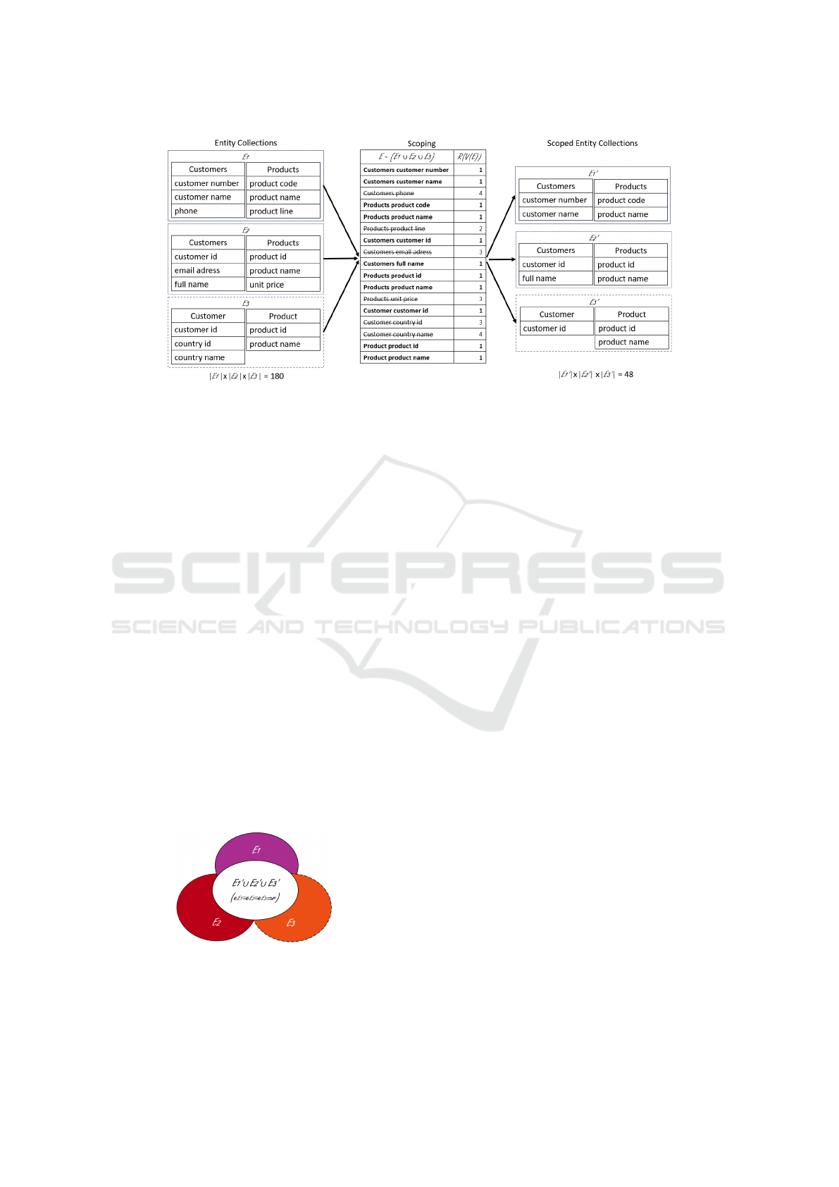
Figure 1: Scoping of multi-sourced Entity Collections (Example).

the end of the EL process. For example, as the entity

collections become larger due to the rise in Volume,

we observe an increase in heterogeneity and a de-

crease in Veracity. Figure 2 illustrates the increasing

heterogeneity represented by the colored entity col-

lections represented as ovals with unlinkable entities,

while the linked ones are shown in the white overlap-

ping oval. Scoping seeks entities with linkages repre-

sented in the overlapping oval. The contributions of

this paper are:

• We introduce scoping, a novel and integral phase

of Entity Linkage, positioned right after the sig-

nature and before the blocking phase (Figure 3),

improving the quality of the search space of pair

candidates (Section 3).

• We create entity ranking methods for scoping by

relating them to anomaly detection and adapt Z-

score, LOF, PCA, autoencoders, and ensembles as

entity ranking methods (Section 3.2).

• We evaluate our scoping approach based on ad-

ditional performance metrics on a new real-world

dataset ”OC3-HR” for multi-sourced Entity Link-

age (Section 4).

Figure 2: Visualisation of Scoping of multi-sourced Entity

Collections based on Figure 1.

2 RELATED WORK

Traditional ER workﬂows consist of three sequential

phases. In the signature phase, a numerical embed-

ding strategy applies to all entity proﬁles. The vec-

torization of an entity proﬁle, such as an attribute

in a relational database named “customer address”

can be based on tf-idf (Paulsen et al., 2023), the ag-

gregation of pre-trained Word2Vec embeddings such

as Glove or FastText (Cappuzzo et al., 2020). Fur-

ther techniques combine words via sequence model-

ing, transformers, and self-supervised models (Brun-

ner and Stockinger, 2020), (Thirumuruganathan et al.,

2021), (Azzalini et al., 2021), (Zeakis et al., 2023).

The blocking phase generates a set of likely match-

ing entity proﬁles into buckets. This phase rarely

incorporates any further knowledge infusion except

query tokens that vary with hyperparameter settings

such as the size of the buckets and parallelization

settings on hardware. Respective algorithms use di-

mensionality reduction techniques (PCA, t-SNE) to

reduce the signature length. Then, nearest-neighbor

algorithms (ENNs such as Hierarchical Clustering,

K-Means, DBSCAN) (Azzalini et al., 2021) or ap-

proximate nearest-neighbor algorithms using hash in-

dexing methods (ANNs such as LSH with FAISS

or SCANN implementation) are applied to generate

buckets of similar entities (Zeakis et al., 2023), (John-

son et al., 2019), (Guo et al., 2020).

Finally, the ﬁltering phase constructs a set of ver-

iﬁed linkages of matching entity proﬁles. This phase

examines every inter-bucket pair and ﬁlters out un-

wanted linkages whose similarity is below a similarity

threshold while keeping those that exceed the thresh-

old. Filtering is optional and applies to the Carte-

sian set between entities within a blocking-generated

ICEIS 2024 - 26th International Conference on Enterprise Information Systems

108

Figure 3: Entity Linkage Workﬂow with Scoping.

bucket (Koutras et al., 2021), (Traeger et al., 2022).

3 SCOPING

Scoping combines a ranking algorithm with a tun-

able threshold for generating streamlined entity col-

lections. We assume a schema-aware, multi-sourced

and unsupervised entity linkage environment. First,

we provide an overview of the notations of this sec-

tion in Table 1.

3.1 Scoping Deﬁnition

In entity linkage, we aim to ﬁnd the set of linked entity

proﬁles in which entities share the same real-world

entity representation L(E) = {(e

) : e

∈ E

and

∈ E

so that e

≡ e

⇒ r} where E

∈ E be-

tween entity collections.

Scoping utilizes the entity signatures v

, the pre-

viously vectorized entity proﬁles processed by the

Entity Signature phase V (E). Before applying the

actual scoping method, an Entity Ranking algorithm

R (V (E)) computes an entity score for each entity

signature, returning the tuple (e

) where s

is the

score of entity proﬁle e

. The ranking algorithms pre-

sented in Section 3.2 categorize entity proﬁles with

lower scores as linkable and higher scores as unlink-

able in comparison to each other. The actual scoping

algorithm S, ﬁrst, sorts the entity score tuples (e

)

in descending order so that s

i+1

. Secondly, the al-

gorithm ﬁlters the entity score tuples to identify and

prioritize top-ranked entities with lower scores. We

provide a single conﬁgurable threshold p ∈ [0,1] for

the scoping algorithm that represents a radius (white

overlapping space in Figure 2) for selecting linkable

entities depending on the scores. The output of scop-

ing generates a new subset E

′

⊆ E with fewer entity

proﬁles selected from the original entity collection.

Subsequently, blocking the entity proﬁles across E

′

instead of E results in higher quality entity pair candi-

dates, resulting in less computational resources (space

and time). Scoping generally differs in comparison to

blocking in the sense that it aims to generate a sub-

set entity collection E

′

∈ E without compromising

the set of linkages L(E

′

) ≡ L(E) regardless of the

blocking sequence.

Figure 1 shows the effect of scoping on the orig-

inal collection, in which a ranking algorithm com-

putes a score for each entity and scopes 11 out of the

17 top-scored entities (p = 0.65). Unlinkable entities

like “phone” and “country id” are omitted. With the

scoped collections, we go down from 180 to 48 po-

tential linkages without missing a single true linkage.

3.2 Ranking Methods in Scoping

In Section 3.1, we describe that the ranking methods

R (V (E)) process the entity signatures to compute an

entity score tuple (e

) used to scope a relative por-

tion of E based on p in order to generate a subset of

entity collections E

′

. It is worth noting that the size

of the data input in scoping is linear in the number of

entity proﬁles |E

| + |E

...

| + |E

| and not the Carte-

sian product (brute force) between all possible entity

pairs between entity collections |E

| × |E

...

| × |E

Now, we present two modiﬁed outlier algorithms that

compute anomaly scores v

for each entity signature.

Then, we introduce our novel encoder-decoder-based

anomaly detection algorithms. We provide a compu-

tational complexity analysis for each of these algo-

rithms that we evaluate in Section 4.

Z-Score: It is a statistical measure to quantify the

entity’s degree of dispersion. Its anomaly score

implies how many standard deviations σ an entity

signature differs from the mean µ of all entity signa-

tures (e

) = ||

−µ)

||. The Z-Score is computed

per dimension of the entity signature and results in

positive and negative ﬂoating values. Subsequently,

the mean of the absolute (positive) dimension-based

Z-scores along with the entity signature represents

the entity score. The time complexity for computing

the Z-scores is O(|E| · ¯v).

Local Outlier Factor (LOF): It is a density-based

method that quantiﬁes the local deviation of a data

point from its neighborhood. The locality of the

anomaly score depends on the degree of isolation

(e.g., Euclidean or Cosine) between the entity

signature and the surrounding entity signatures

given by k-nearest neighbors. By comparing the

local distances of one entity’s signature to the local

densities of its surroundings, those with substantially

lower densities are considered to be outliers. We

highlight that LOF requires k as a hyperparameter

Scoping: Towards Streamlined Entity Collections for Multi-Sourced Entity Resolution with Self-Supervised Agents

109

input representing the number of neighborhoods.

The value of k directs the number of global linkages

between entities and, therefore, highly inﬂuences

the local density scores. The time complexity for

computing the LOF is O(|E| · ¯v · k). We refer to the

original paper (Breunig et al., 2000) for more details.

Encoder-Decoder: Next, we propose a novel method

based on self-supervised encoder-decoder models to

implement scoping. A main challenge in anomaly de-

tection is the high dimensional space that occurs in the

vectorized entities (signatures). In the past, anomaly

detection with neural networks has received a lot of

attention (Gong et al., 2019), (Bank et al., 2021),

(Ruff et al., 2021), (Ilyas and Rekatsinas, 2022). The

effect of learning a generative model and using it to

detect anomalies has not yet been utilized within the

Entity Linkage research space, and therefore, it moti-

vates this work.

Once an encoder-decoder model is trained, fre-

quent entities that are similar and appear to exhibit

linkages pass the autoencoder with a lower recon-

struction error. The reason for this is a bottleneck

that appears in encoder-decoder algorithms, forcing

the model to focus on recurring entities during the

training rather than on rare anomalous ones. We adopt

this criterion for identifying entities with a high re-

construction error as entities out of the linkage bound.

To leverage an entity score of these methods for the

scoping framework, a wrapped-up agent computes the

mean squared error between the original and decoded

entity signatures. We illustrate the functionality in

Figure 4 and translate this model to an EL agent, as

it provides feedback on the adaptability of entities for

the linkage task based on a low or high reconstruc-

tion error. Additionally, the model of agents can be

reused to rank entities of newly adapted collections.

The beneﬁt of using a trained model is that a holis-

tic recomputation, such as needed for the Z-Score or

LOF method, might not always be necessary. This ap-

proach can improve efﬁciency and save resources via

Figure 4: Agent for Entity Ranking in Scoping.

task transferability in EL pipelines.

Principal Component Analysis (PCA): Applying PCA

onto the entity signatures transforms them into a

lower-dimensional space. The reduced space should

also capture relevant patterns. Each principal com-

ponent in PCA quantiﬁes the importance of the dis-

parity of entities along its dimension based on lin-

ear hyperplanes. This is useful, as the signatures

of unlinkable entities may exhibit unique patterns in

high-dimensional space. PCA can be reused for scop-

ing new entity collections by applying the model and

comparing the mean squared error. We now present

the PCA algorithm for scoping:

Data: V (E) = (v

) Entity Signatures

Result: R (V (E)) = (e

) Entity Scores

X = scaler(0,1).ﬁt((v

));

µ = mean(X);

//along dimensions;

pca = sklearn.PCA(nc).ﬁt(X);

//singular value decomposition;

Z = pca.transform(X);

X = (Z· pca.components) + µ;

return (s

) ⇐ MSE(X ,

X);

Algorithm 1: Entity Ranking R with PCA.

The ﬁrst line casts an optional [0..1] normalization

along the entity signature dimensions, transforming

the set of entity signatures (v

) to the input data set

X. As entity signatures contain both negative and

positive values along the dimensions, normaliza-

tion simpliﬁes the subsequent mean and similarity

calculations. X is a |E| × ¯v matrix in which |E|

represents the number of entities of a collection and

¯v represents the dimensional length of the entity

Table 1: Notation Table.

Notation Meaning

Entity Proﬁle

source

= (e

...

) Entity Collection

≡ e

...

(≡ e

) ⇒ r) Real-world Entity

E = E

∪ E

...

∪ E

Uniﬁed Entity Collection

V (E) = (v

) Entity Signature

R (V (E)) = (e

) Entity Ranking (score-tuple)

S((e

), p) = {(e

) : ∀s

i+1

∧ |(e

)| × p} = E

′

Entity Scoping (threshold)

B(E) = {(e

) : e

∈ E

∧ e

∈ E

} where E

∈ E Entity Blocking (brute-force)

L(E) = {(e

) : e

∈ E

∧ e

∈ E

≡ e

⇒ r} where E

∈ E Entity Linkage

ICEIS 2024 - 26th International Conference on Enterprise Information Systems

110

signature. In the second step, we compute the µ

vector of the mean along each dimension. Thirdly,

we initialize PCA with the number of components

given by the hyperparameter nc, subtract µ from

each (normalized) vector signature X , and compute

the singular value decomposition for each principal

component with the same vector length as ¯v. Sub-

sequently, we can now project the input data set X

onto the lower-dimensional principal components,

resulting in the encoded |E| × nc matrix we deﬁne as

Z. Finally, we cast the decoder operation to generate

X. This involves reversing the dot-product between

Z and principal components plus the entity-wise

addition of the mean µ. Lastly, we compute the

mean-squared error (MSE) between X and

X and

utilize these as the entity scores (s

). The time com-

plexity for PCA is O(|E| · ¯v

+ ¯v

). We refer to the

tutorial paper (Shlens, 2014) for more details on PCA.

Autoencoders: They are a special type of neural

networks trained to encode data on a meaningful rep-

resentation and reversely decode it back to its original

state. These models are considered self-supervised

as the data serves both as training input and output.

Similar to PCA, we follow the assumption that a

trained autoencoder learns relevant patterns more

efﬁciently of normally distributed entity signatures

but not for anomalous and unlinkable ones. More-

over, autoencoders with one latent layer and linear

activation functions generalize PCA. In the following

section, we provide a summary of autoencoders in the

context of anomaly detection using the reconstruction

error for scoping. More details on autoencoders can

be found in the survey by (Bank et al., 2021).

We formally denote the encoder function as

A(V (E) = X ) ⇒ Z mapping the set of the normal-

ized entity signatures into a latent lower-dimensional

representation. The decoder function B(Z) ⇒

X aims

to transform the latent representation into the original

input. Both the functions of A and B are trained over

a number of epochs ep in order to minimize the mean

reconstruction error converging to

arg min

A,B

[MSE(X,B(A(X )))]

Contrary to PCA, normalization of the entity sig-

natures not only simpliﬁes the computation but allows

the use of non-linear activation functions. Both the

encoder and decoder functions can, therefore, con-

struct more elegant and superior non-linear hyper-

planes. At the same time, non-linear hyperplanes

tend to overﬁt. For this reason, different types of

regularization beyond the lower-dimensional bottle-

neck must be considered depending on the number

of entities |E|, signature length ¯v, and degree of de-

viations. Various possible conﬁgurations of the au-

toencoder may consider the network’s depth or shal-

lowness, the number of epochs, layers, neurons, acti-

vation functions, optimization algorithms, loss, and

validation sampling conﬁgurations. The computa-

tional time complexity depends on those architectural

choices; therefore, providing a O() notation varies

and is dependent on each different conﬁguration. Due

to the rising time complexity of backpropagating the

weights of each neuron in each hidden layer over

multiple epochs, we assume autoencoders to have a

higher time complexity compared to the previously

presented ranking methods. In the scoping context,

we generally recommend preventing overﬁtting with

regularization, as such a model would generate iden-

tical entity scores that are not useful for scoping.

4 EVALUATION

We evaluate the scoping approach on a real-world

multi-sourced entity linkage dataset. We ﬁrst

present the performance metrics we use, then we

describe the dataset, elaborate on chosen signa-

ture strategies, and the conﬁguration of the rank-

ing methods. All experiments were performed

in Python Jupyter hosted by Google Collabora-

tory

. The dataset and code are available at

https://github.com/leotraeg/scoping.

Performance Metrics: To measure the effectiveness

of the algorithms for generating scoped entity collec-

tions E

′

from the original ones E, we adopt typical

metrics used in ER.

• Reduction Ratio (RR(E

′

,E)) reﬂects the time efﬁ-

ciency in scoping without relevance to the ground

truth of linkages. It expresses the reduction in the

number of entity comparisons between the scoped

entity collections and the original ones:

1 − ||B(E

′

...

′

)||/||B(E

...

)||.

• Pair Completeness (PC(E

′

,E)) estimates the

number of potentially true entity linkages within

the scoped entity collections with respect to the

number of the ground truth entity linkages within

the original entity collections:

||L(E

′

...

′

)||/||L(E

...

)||.

• Harmonic-Mean RR-PC (HM(E

′

,E))) represents

a combined metric between the two competing

objectives of reduction ratio and pair complete-

ness.

2·RR·PC

RR+PC

The threshold p affects the collections of scoped

entities E

′

in a major way. Knowing its value before-

https://colab.research.google.com

Scoping: Towards Streamlined Entity Collections for Multi-Sourced Entity Resolution with Self-Supervised Agents

111

Table 2: Description of OC3-HR: a multi-sourced entity linkage dataset with relational database schemas.

Entity Collections (E

− E

) #Tables #Attributes |E

| × |E

| #Attribute Linkages

Domain-speciﬁc

∑

OC3 18 142 6617 47

OC-Oracle – OC-MySQL 15(7+8) 102(43+59) 2537 19

OC-Oracle – OC-HANA 10(7+3) 83 (43+40) 1720 16

OC-MySQL – OC-HANA 11(8+3) 99 (59+40) 2360 12

Domain-agnostic

∑

OC3-HR 25 177 11587 62

HR-Oracle – OC-Oracle 14 (7+7) 78 (35+43) 1505 0

HR-Oracle – OC-MySQL 15 (7+8) 94 (35+59) 2065 14

HR-Oracle – OC-HANA 10 (7+3) 75 (35+40) 1400 1

hand implies knowing the ground truth of entity link-

ages. As this is not true in reality, we propose to adjust

p as an engineering task aiming to yield better perfor-

mance by introducing two new metrics using the Area

Under Curve and comparing them.

• Area Under Curve PC APC(E

′

,E) evaluates the

entity scoring utility in scoping. The more entity

pairs that are correctly found with increasing p,

the higher the single-valued APC metric. A higher

APC for one ranking method allows more con-

ﬁdence in lowering the p threshold without time

considerations.

• Area Under Curve HM AHM(E

′

,E) helps to

quantify the trade-off between the reduction ratio

and pair completeness across all p thresholds. A

higher AHM recommends a more robust scoping

approach considering both the pair completeness

and time efﬁciency.

Schemas and Experiments: The datasets that we

use contain only schema information from Oracle,

MySQL, and SAP HANA, without instance data.

First, we perform a set of experiments on a domain-

speciﬁc set of order-customer (OC) schemas with

47 true inter-schema attribute linkages out of 6617

attribute-pair candidates. Then, we conduct the same

experiments on a domain-agnostic set of schemas by

extending the domain-speciﬁc schemas with a hu-

man resources (HR) schema. We annotate 15 ad-

ditional inter-schema attribute pairs since the OC-

MySQL schema contains attribute linkages between

employees and ofﬁces. Consequently, the domain-

agnostic setting contains 11587 attribute pair candi-

dates, of which 62 are considered true. We provide a

detailed summary of the dataset in Table 2.

Signature: We uniformly preprocess the textual de-

scriptions of each entity across all collections by

concatenating the table and attribute names, splitting

concatenated words, and removing repetitive words.

Based on the comparative analysis by (Zeakis et al.,

2023), we aggregate static Glove embeddings trained

on Common Crawl without out-of-vocabulary vec-

tor retrievals (Pennington et al., 2014) and use Sen-

tence Transformer Bert (gtrt5-base) (Reimers and

Gurevych, 2019) as the best dynamic strategy.

Ranking: We use the following conﬁgurations for the

ranking methods:

• Z-Score: We use the default implementation of

the SciPy

library.

• LOF: We import the sklearn neighbors library

and specify the number of neighbors k = 15 as

these are the average number of linkages between

the entity collections.

• PCA: We use the Lapack SVD implementation of

the sklearn decomposition library

and use nc = 2

(number of principal components) as we deal with

a small size of |E|.

• AE: We use the Keras library and conﬁgure an au-

toencoder with three intermediate layers to extend

the network complexity to PCA. We use rectiﬁed

linear units (ReLUs), Adam as the optimizer, the

mean squared error (MSE) as the loss function,

and a shufﬂed test-train split of 20%. To pre-

vent identity functions, we deﬁne the small size

of ten epochs (ﬁxed early stopping) but initialize

the model ten times and sum up each entity’s MSE

to stabilize the ﬁnal entity score.

• Ensemble: We take the mean score across the

normalized entity score tuples (e

) of the best-

performing conﬁgurations of Z-Score, LOF, PCA,

and AE based on APC, AHM

, and AHM

. In

this regard, an equally weighted ensemble of en-

tity scores works similarly to a random forest (su-

pervised) or consensus clustering (unsupervised).

Blocking: Blocking primarily affects the time reduc-

tion ratio, while scoping affects the completeness of

entity linkage pairs. To show this distinction, we em-

ploy two blocking modules: the ﬁrst is a simplistic

entity blocking module B that schedules all potential

inter-source-linkages (Cartesian product) between the

(scoped) entity collections at point p. The second one

https://docs.scipy.org/doc/scipy

https://scikit-learn.org

ICEIS 2024 - 26th International Conference on Enterprise Information Systems

112

Table 3: Scoping conﬁgurations and Area Under Curve PC and HM performances on OC3-HR dataset.

Scoping Domain-speciﬁc Domain-agnostic

V Signature R Ranking R Parameter APC AHM

AHM

APC AHM

AHM

Glove Z-score none 52.36 47.30 53.69 54.21 44.81 53.46

gtrt5 Z-score none 60.52 46.82 54.11 50.57 45.06 53.61

Glove LOF k = 15 54.37 45.69 52.53 52.62 44.60 53.82

gtrt5 LOF k = 15 61.59 48.19 55.40 57.69 46.91 56.20

Glove PCA n = 2 53.03 45.38 52.13 53.61 45.33 54.32

gtrt5 PCA n = 2 61.80 49.06 56.17 56.81 46.94 55.79

Glove AE 610,300,10,300,610 52.69 47.33 53.83 49.97 44.95 53.73

gtrt5 AE 778,300,10,300,778 64.05 49.45 56.73 57.58 47.11 56.02

Ensemble max

APC,AHM

,AHM

63.86 50.92 58.10 58.81 47.45 56.38

is the efﬁcient locality-sensitive hashing-based sim-

ilarity search blocking module F implemented with

the Python package FAISS

(Papadakis et al., 2022)

(Paulsen et al., 2023), (Zeakis et al., 2023). This

blocking scheme queries each entity signature and

outputs a maximum of k = 50 linkage candidates

based on the L2-distanced nearest neighbors.

Scoping Results and Discussion: We evaluate the

scoping approach on the OC3-HR dataset. We re-

port the AUC metrics for the pair completeness (APC)

and the harmonic mean for the brute force (AHM

)

and FAISS-based (AHM

) blocking modules. The

results are based on the entity signature V , ranking

method R , and parameter conﬁgurations summarized

in Table 3. The best result per ranking method is

highlighted in bold. Figure 5 and 6 plot the best-

performing stand-alone and ensemble conﬁgurations

for APC and AHM with the performance (y-axis) of

the time reduction ratio (yellow), pair completeness

(blue), and the harmonic mean (green) on the increas-

ing relative threshold parameter p (x-axis). Generally,

Sentence Transformer Bert (gtrt5) signatures outper-

form word2vec (Glove) with minor exceptions for the

Z-Score method. It is worth noting that we also com-

pared two blocking methods, showing that the FAISS-

based one improved in computational time reﬂected

in AHM

. However, none of them had any effect on

the number of true linkages as measured in APC.

We ﬁrst discuss the results obtained for the

domain-speciﬁc dataset. The best-performing stand-

alone model for APC and AHM is the autoencoder

with gtrt5 signatures. We explain the 2.25% domain-

speciﬁc APC improvement for autoencoders with the

ensembling training nature: autoencoders’ compres-

sion and decompression functions are trained over

multiple epochs with a shufﬂed train-test split of en-

tity signatures. On the contrary, the ensemble method

yields the best performance for AHM.

https://github.com/facebookresearch/faiss

We now discuss the results obtained for the domain-

agnostic dataset. Among the signature strategies,

all ranking methods and conﬁgurations perform the

best with gtrt5 signatures except for Z-Score in APC.

The best stand-alone APC performance is achieved

by LOF, falling 1% below the ensemble. For the

domain-agnostic dataset, the ensemble method per-

forms best in both AHM and APC. In general, the

domain-agnostic dataset contains several pairs that

are not linkable due to the fact that the schemas do not

reﬂect similar domains. Although the true linkages

are still captured in the domain-agnostic schemas, it

is expected to observe a decrease in the performance

metrics due to the dissimilarity of the schemas.

Summary: Evaluations on multi-sourced schemas

show that autoencoders with gtrt5 signatures perform

best in the domain-speciﬁc entity linkage task. We

highlight that this scoping conﬁguration reduces the

search space to 77% of entities and still contains all

linkages. The impact of the ranking method is more

relevant for the domain-speciﬁc setting rather than

the domain-agnostic setting. Generally, ensembling

the entity scores of different ranking methods can

yield more robust results for both APC and AHM. Fi-

nally, all scoping conﬁgurations for both the domain-

speciﬁc and agnostic settings intersect with the graph

of the time reduction ratio at 50% (x-axis) and the pair

completeness at around 75% (y-axis). This means

that scoping can reduce the original set of entity col-

lections when the time for comparisons is limited and

still retain a high portion of true linkages.

5 CONCLUSION

This paper introduced scoping, a new phase in the EL

pipeline that ranks entities and generates a subset E

′

of the raw entity collections E while leaving intact

the major set of true linkages. We have shown that

Scoping: Towards Streamlined Entity Collections for Multi-Sourced Entity Resolution with Self-Supervised Agents

113

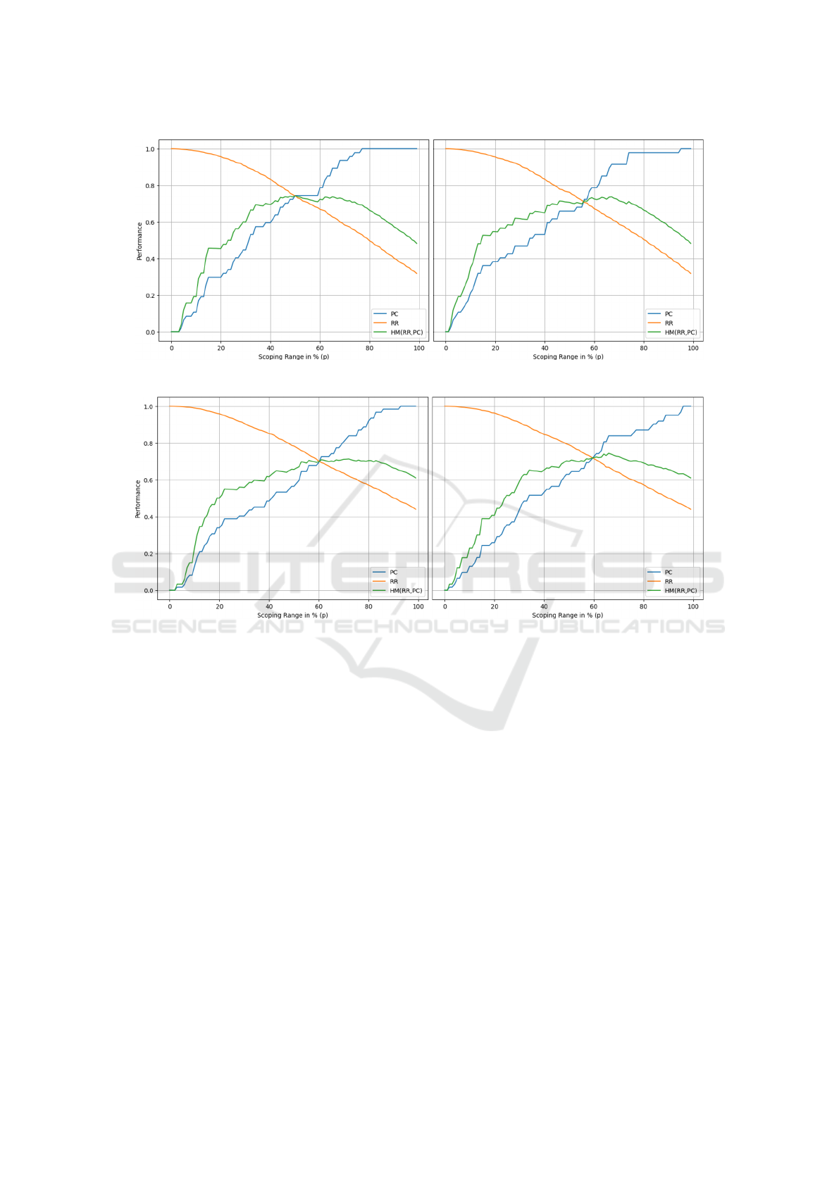
Figure 5: RR, PC, and HM performance on domain-speciﬁc OC3 dataset (left: AE with gtrt5 and right: ensemble).

Figure 6: RR, PC, and HM performance on domain-agnostic OC3-HR dataset (left: LOF with gtrt5 and right: ensemble).

models learning to compress and decompress entities

from multiple data sources can be used to scope out

linkable entities with better or almost equal perfor-

mance compared to existing ranking methods. We

see the various autoencoder network conﬁgurations

as a strength to better adapt to different numbers of

entities |E|, the dimensionality of entity signatures

¯v, and the degree of domain speciﬁcity. Moving on

to the potential advantages of self-supervised models,

we highlight that PCA and the autoencoder model can

be reused to scope new incoming entity collections.

In future work, we plan to investigate autoencoders

enriched with a multi-modal network to incorporate

textual descriptions and instances from entity proﬁles.

REFERENCES

Azzalini, F., Jin, S., Renzi, M., and Tanca, L. (2021). Block-

ing Techniques for Entity Linkage: A Semantics-

Based Approach. Data Science and Engineering,

6(1):20–38.

Bank, D., Koenigstein, N., and Giryes, R. (2021). Autoen-

coders. arXiv:2003.05991 [cs, stat].

Breunig, M. M., Kriegel, H.-P., Ng, R. T., and Sander, J.

(2000). LOF: identifying density-based local outliers.

ACM SIGMOD Record, 29(2):93–104.

Brunner, U. and Stockinger, K. (2020). Entity match-

ing with transformer architectures - a step forward in

data integration. Medium: application/pdf Publisher:

OpenProceedings.

Cappuzzo, R., Papotti, P., and Thirumuruganathan, S.

(2020). Creating Embeddings of Heterogeneous Re-

lational Datasets for Data Integration Tasks. In Pro-

ceedings of the 2020 ACM SIGMOD International

Conference on Management of Data, SIGMOD ’20,

pages 1335–1349, New York, NY, USA. Association

for Computing Machinery.

Gong, D., Liu, L., Le, V., Saha, B., Mansour, M. R.,

Venkatesh, S., and Hengel, A. v. d. (2019). Mem-

orizing Normality to Detect Anomaly: Memory-

augmented Deep Autoencoder for Unsupervised

Anomaly Detection. arXiv:1904.02639 [cs].

Guo, R., Sun, P., Lindgren, E., Geng, Q., Simcha, D.,

Chern, F., and Kumar, S. (2020). Accelerating large-

scale inference with anisotropic vector quantization.

ICEIS 2024 - 26th International Conference on Enterprise Information Systems

114

Ilyas, I. F. and Rekatsinas, T. (2022). Machine Learning and

Data Cleaning: Which Serves the Other? Journal of

Data and Information Quality, 14(3):13:1–13:11.

Johnson, J., Douze, M., and J

egou, H. (2019). Billion-scale

similarity search with GPUs. IEEE Transactions on

Big Data, 7(3):535–547.

Koutras, C., Siachamis, G., Ionescu, A., Psarakis, K.,

Brons, J., Fragkoulis, M., Loﬁ, C., Bonifati, A.,

and Katsifodimos, A. (2021). Valentine: Evaluating

Matching Techniques for Dataset Discovery. In 2021

IEEE 37th International Conference on Data Engi-

neering (ICDE), pages 468–479. ISSN: 2375-026X.

Lerm, S., Saeedi, A., and Rahm, E. (2021). Extended

Afﬁnity Propagation Clustering for Multi-source En-

tity Resolution. BTW 2021.

Papadakis, G., Fisichella, M., Schoger, F., Mandilaras, G.,

Augsten, N., and Nejdl, W. (2022). How to reduce the

search space of Entity Resolution: with Blocking or

Nearest Neighbor search? arXiv:2202.12521 [cs].

Paulsen, D., Govind, Y., and Doan, A. (2023). Sparkly:

A Simple yet Surprisingly Strong TF/IDF Blocker for

Entity Matching. Proceedings of the VLDB Endow-

ment, 16(6):1507–1519.

Pennington, J., Socher, R., and Manning, C. D. (2014).

Glove: Global vectors for word representation. In

EMNLP, volume 14, pages 1532–1543.

Reimers, N. and Gurevych, I. (2019). Sentence-bert: Sen-

tence embeddings using siamese bert-networks. In

Proceedings of the 2019 Conference on Empirical

Methods in Natural Language Processing. Associa-

tion for Computational Linguistics.

Ruff, L., Kauffmann, J. R., Vandermeulen, R. A., Mon-

tavon, G., Samek, W., Kloft, M., Dietterich, T. G., and

uller, K.-R. (2021). A Unifying Review of Deep

and Shallow Anomaly Detection. Proceedings of the

IEEE, 109(5):756–795. arXiv:2009.11732 [cs, stat].

Shlens, J. (2014). A Tutorial on Principal Component Anal-

ysis. arXiv:1404.1100 [cs, stat].

Thirumuruganathan, S., Li, H., Tang, N., Ouzzani, M.,

Govind, Y., Paulsen, D., Fung, G., and Doan, A.

(2021). Deep learning for blocking in entity match-

ing: a design space exploration. Proceedings of the

VLDB Endowment, 14(11):2459–2472.

Traeger, L., Behrend, A., and Karabatis, G. (2022). In-

teplato: Generating mappings of heterogeneous rela-

tional schemas using unsupervised learning. In 2022

International Conference on Computational Science

and Computational Intelligence (CSCI), pages 426–

431.

Zeakis, A., Papadakis, G., Skoutas, D., and Koubarakis, M.

(2023). Pre-Trained Embeddings for Entity Resolu-

tion: An Experimental Analysis. Proceedings of the

VLDB Endowment, 16(9):2225–2238.

Scoping: Towards Streamlined Entity Collections for Multi-Sourced Entity Resolution with Self-Supervised Agents

115