Can a Simple Approach Perform Better for Cross-Project Defect
Prediction?
Md. Arman Hossain
1
, Suravi Akhter
2
, Md. Shariful Islam
3
, Muhammad Mahbub Alam
4
and Mohammad Shoyaib
1
1
Institute of Information Technology, University of Dhaka, Dhaka, Bangladesh
2
Department of Computer Science and Engineering, University of Liberal Arts Bangladesh, Dhaka, Bangladesh
3
Department of Mathematics, University of Dhaka, Dhaka, Bangladesh
4
Department of Computer Science and Engineering, Islamic University of Technology, Gazipur, Dhaka, Bangladesh
Keywords:
Cross-Project Defect Prediction, Transfer Learning, Second Order Statistics.
Abstract:
Cross-Project Defect Prediction (CPDP) has gained considerable research interest due to the scarcity of
historical labeled defective modules in a project. Although there are several approaches for CPDP, most
of them contains several parameters that need to be tuned optimally to get the desired performance. Often,
higher computational complexities of these methods make it difficult to tune these parameters. Moreover,
existing methods might fail to align the shape and structure of the source and target data which in turn
deteriorates the prediction performance. Addressing these issues, we investigate correlation alignment for
CPDP (CCPDP) and compare it with state-of-the-art transfer learning methods. Rigorous experimentation
over three benchmark datasets AEEEM, RELINK and SOFTLAB that include 46 different project-pairs,
demonstrate its effectiveness in terms of F1-score, Balance and AUC compared to six other methods TCA,
TCA+, JDA, BDA, CTKCCA and DMDA JFR. In terms of AUC, CCPDP wins at least 32 and at most 42 out
of 46 project pairs compared to all transfer learning based method.
1 INTRODUCTION
Software Defect Prediction (SDP) has achieved
noticeable research attention because an early
identification of defects is essential for cost efficient
software development and enhanced customer
satisfaction. It helps to allocate the testing resources
timely and efficiently (Menzies et al., 2010). When
a particular project is rich enough with historical
labeled defect modules, a traditional classification
algorithm can be easily employed for predicting
defects in new modules. This process is known as
Within Project Defect Prediction (WPDP) (Herbold
et al., 2018; Akhter et al., 2023). In reality, due
to lack of expertise, time and funding, most of
the projects often do not contain previous labeled
defective data, and thus, WPDP is less attracted by
researchers nowadays. On the other hand, Cross-
Project Defect Prediction (CPDP) is a process that
does not require project specific historical data. It
learns from existing labeled project(s) (source) which
is different but related to the project for prediction
(target), that makes CPDP advantageous over WPDP.
However, although source and target are related, their
distribution may differ due to data collection time,
software version, configuration etc. Unfortunately,
directly applying traditional classification algorithms
do not perform well in such cases.
To solve this issue, filter (Turhan et al., 2009;
Peters et al., 2013) and Transfer Learning (TL) based
methods (Liu et al., 2019; Qiu et al., 2019; Xu
et al., 2019) are usually used for CPDP. Filter-
based methods discard the dissimilar instances from
the source project considering target instances. In
contrast, TL-based methods leverage all instances
to identify transformation matrices. These matrices
are then utilized to transform either source or target
or both data into a separate space to maximize the
similarity between source and target. TL-based
methods have gained popularity over filter-based
methods because the discarded instances may take
away valuable information from the training projects.
Transfer Component Analysis (TCA) (Pan et al.,
2010) is one of the pioneer method for TL that
328
Hossain, M., Akhter, S., Islam, M., Alam, M. and Shoyaib, M.
Can a Simple Approach Perform Better for Cross-Project Defect Prediction?.
DOI: 10.5220/0012617300003687
Paper published under CC license (CC BY-NC-ND 4.0)
In Proceedings of the 19th International Conference on Evaluation of Novel Approaches to Software Engineering (ENASE 2024), pages 328-335
ISBN: 978-989-758-696-5; ISSN: 2184-4895
Proceedings Copyright © 2024 by SCITEPRESS – Science and Technology Publications, Lda.

finds a shared subspace to reduce the Maximum
Mean Discrepancy (MMD) between the projected
source and target project. TCA+ (Nam et al.,
2013) introduced different types of normalization
before applying TCA in CPDP. Two-Phase Transfer
Learning (TPTL) (Liu et al., 2019) extends TCA+
by choosing the best suited source project from a
set of given projects. Considering both marginal
and conditional distributions Joint Distribution
Adaptation (JDA) (Long et al., 2013) has been
proposed which is further utilized by Balanced
Distribution Adaptation (BDA) (Xu et al., 2019)
for CPDP by balancing the importance of marginal
and conditional distributions. Recently, Cost-
sensitive Transfer Kernel Canonical Correlation
Analysis (CTKCCA) (Li et al., 2018) and Joint
Feature Representation with Double Marginalized
Denoising Autoencoders (DMDA JFR) (Zou et al.,
2021) have been proposed to solve class imbalance
problem, capture nonlinear correlation and minimize
distribution difference between target and source.
In addition DMDA JFR reduces marginal and
conditional distributions by preserving local and
global feature structure as well and thus, ensures a
reasonable performance.
All the aforementioned methods minimize
either marginal or conditional or both distributions
discrepancy between source and target. However, the
minimization involves several parameters which are
computationally expensive to tune. The minimization
of conditional discrepancy requires pseudo labels
of the target modules that might degrade the
model performance (Zou et al., 2021). Moreover,
these methods use symmetric transformation (i.e.,
they use same transformation for both source and
target domain) that might ignore the similarity
between source and target. One of the state-of-
the-art symmetric transformation-based method
is CORrelation ALignment (CORAL) for domain
adaptation (Sun et al., 2017) and is applied in CPDP
(Niu et al., 2021) and heterogeneous CPDP (Li et al.,
2019; Pal and Sillitti, 2022). The respective major
goal of these paper is preprocessing of data prior to
applying CORAL and extend it for heterogeneous
CPDP. However, to the best of our knowledge,
none of these papers investigate the strength of
CORAL in comparison with standard transfer
learning based methods for CPDP. In this paper, we
thoroughly investigate CORAL for Cross-Project
Defect Prediction (CCPDP), a computationally
simple and parameter-free asymmetric approach,
that is based on second order statistic (covariance)
in comparison with the renowned transfer learning
methods such as TCA, TCA+, JDA, BDA, CTKCCA
and DMDA JFR. The key contributions of this paper
are listed below:
1. We provide a justification that a second order
statistics can be applied for transfer learning in
CPDP which can capture the shape and structure
of data effectively and efficiently by utilizing a
second order statistic.
2. We demonstrate the superiority of CCPDP by
extensive experimentation over three benchmark
datasets containing 46 project-pairs by comparing
it with six transfer learning based methods.
2 PRELIMINARIES
In this section, we have introduced the notations
and objective function of CPDP approaches including
TCA, TCA+, JDA, BDA, DMDA JFR and CTKCCA.
2.1 Notations
We denote m as number of features and n
s
, n
t
are
numbers of modules (instances) in source and target
project, respectively. Source project X
s
∈ R
n
s
×m
and
its label Y
s
∈ R
n
s
×1
. Target project X
t
∈ R
n
t
×m
and
its label Y
t
∈ R
n
t
×1
. X = X
T
s
∪X
T
t
∈ R
m×(n
s
+n
t
)
is
a combined project of source and target. p is the
number of latent features. K,W, H, and I are kernel,
projection, centering and identity matrix respectively.
c ∈ {1, 2, . . . ,C} is distinct class label. M
c
is class-
wise MMD matrix where (M
c
)
i j
=
1
n
c
s
2
if X
i
, X
j
∈ X
s
;
1
n
c
t
2
if X
i
, X
j
∈ X
t
; −
1
n
c
s
n
c
t
if X
i
∈ X
s
, X
j
∈ X
t
or X
i
∈
X
t
, X
j
∈ X
s
; otherwise 0, and (M
0
)
i j
=
1
n
2
s
if X
i
, X
j
∈
X
s
;
1
n
2
t
if X
i
, X
j
∈ X
t
; otherwise −
1
n
s
n
t
.
2.2 TCA
TCA learns a nonlinear map φ to project source
modules X
s
i
∈ X
s
and target modules X
t
j
∈ X
t
into a
latent space to reduce squared MMD between them as
defined in Eqn. (1).
Dist(X
s
, X
t
) =∥
1
n
s
n
s
∑
i=1
φ(X
s
i
) −
1
n
t
n
t
∑
j=1
φ

X
t
j

∥
2
H
(1)
where H denotes universal reproducing kernel
Hilbert space. The objective function of TCA is
defined in Eqn. (2).
min
W
tr(W
T
KM
0
KW ) + µtr(W
T
W ), (2)
s.t.W
T
KHKW = I
Can a Simple Approach Perform Better for Cross-Project Defect Prediction?
329

where µ is a regularization parameter, K =

K
SS
K
ST
K
T S
K
T T

is a (n
s
+ n
t
) ×(n
s
+ n
t
) kernel matrix,
K
SS
, K
T T
and K
ST
are the kernel matrices defined by
kernel trick on the data in the source domain, target
domain, and cross domains respectively and W ∈
R
(n
s
+n
t
)×p
linearly transforms K to p dimensional
space where p < n
s
+ n
t
.
2.3 JDA
JDA minimizes differences in both marginal and
conditional distributions between source and target
simultaneously by optimizing Eqn. (3).
min
W
T
XHX
T
W =I
C
∑
c=0
tr(W
T
XM
c
X
T
W ) + µ ∥W ∥
2
F
(3)
where W ∈ R
m×p
, and µ is a regularization parameter.
2.4 BDA
BDA uses a balance factor µ to adaptively adjust
the importance of both the marginal and conditional
distributions. The objective is defined in Eqn. (4)
mintr(W
T
X((1 −µ)M
0
+ µ
C
∑
c=1
M
c
)X
T
X + λ ∥W ∥
2
F
,
(4)
s.t.W
T
XHX
T
W = I, 0 ≤µ ≤ 1.
when µ = 0, BDA only focuses on minimizing the
marginal distribution, and when µ = 1, it focuses on
the conditional distribution.
2.5 CTKCCA
The objective of CTKCCA is to find W
s
∈ R
d×p
and
W
t
∈R
d×p
, where d is low rank feature approximation
of K. The objective function is Eqn. (5)
max
w
s
,w
t
w
T
s
˜
G
ST
w
t
(5)
s.t.w
T
s
˜
G
SS
w
s
= 1, w
T
t
˜
G
T T
w
t
= 1.
where w
i
∈ R
d
is a column vector,
˜
G
SS
=
∑
C
c=1
f (c)

¯
G
c
s

T
¯
G
c
s
,
˜
G
T T
=
¯
G
T
t
¯
G
t
and
˜
G
ST
=
∑
C
c=1
f (c)

¯
G
c
s

T
Γ
c
G
¯
G
t
are (d × d) dimensional
approximation of the kernel matrices K
SS
, K
T T
and
K
ST
, respectively. f (c) describes the weight of the
class c and Γ
c
G
denotes the similarity weight between
¯
G
c
s
and
¯
G
t
.
¯
G
i
is mean centered G
i
.
2.6 DMDA JFR
DMDA JFR captures the global feature structure
using Eqn. (6)
min
W
1
2l(n
s
+ n
t
)
tr[(X −W
˜
X)
T
(X −W
˜
X)] + µ ∥W ∥
2
F
+ E
mar
(
˜
X
s
,
˜
X
t
) + E
con
(
˜
X
s
,
˜
X
t
). (6)
where µ is the regularization parameter,
˜
X denotes the
corrupted version of X (Wei et al., 2018), l is the
number of repeated version of X, E
mar
(
˜
X
s
,
˜
X
t
) and
E
con
(
˜
X
s
,
˜
X
t
) match the marginal and the conditional
cross-project distributions respectively. E
mar
(
˜
X
s
,
˜
X
t
)
is defined in Eqn. (7)
E
mar
(
˜
X
s
,
˜
X
t
) = W
T
˜
X
T
s
Z
Sl
˜
X
s
W +W
T
˜
X
T
t
Z
T l
˜
X
t
W
−2W
T
˜
X
T
s
Z
ST l
˜
X
t
W. (7)
where Z
Sl
=
1
n
2
s
I
n
s
, Z
T l
=
1
n
2
t
I
n
t
, and Z
ST l
=
1
n
s
n
t
I
n
s
×n
t
.
E
con
(
˜
X
s
,
˜
X
t
) is defined in Eqn. (8)
E
con
(
˜
X
s
,
˜
X
t
) = W
T
˜
X
T
s
Z
c
Sl
˜
X
s
W +W
T
˜
X
T
t
Z
c
T l
˜
X
t
W
−2W
T
˜
X
T
s
Z
c
ST l
˜
X
t
W (8)
To capture local structure with label c DMDA JFR
follows Eqn. (9)
min
W
1
2l(n
s
+ n
t
)
c
tr[(X
c
−W
c
˜
X
c
)
T
(X
c
−W
c
˜
X
c
)]
+ µ ∥W
c
∥
2
F
+E
mar
(
˜
X
s
c
,
˜
X
t
c
). (9)
where X
c
= X
c
s
∪X
c
t
the subset of class c data from
both source and target domain.
3 APPROACH
It is well known that the utilization of covariance in
transfer learning can efficiently capture the structure
of data. (Zhang et al., 2020). This inspires us to adopt
CORrelation ALignment (CORAL) for cross-project
defect prediction.
3.1 Correlation Alignment for
Cross-Project Defect Prediction
To capture domain structure using feature
correlations, CCPDP follows correlation alignment
to minimize distribution difference by aligning the
second-order statistics, i.e., the covariance matrices
of source and target projects without requiring any
pseudo-label. The objective of CCPDP is to find
a linear transformation matrix W that minimizes
Frobenius norm defined as follows
∥W
T
C
s
W −C
t
∥
2
F
, (10)
ENASE 2024 - 19th International Conference on Evaluation of Novel Approaches to Software Engineering
330

Figure 1: Overall process of CCPDP.
where C
s
=
1
n
s
−1
X
T
s
H
s
X
s
and C
t
=
1
n
t
−1
X
T
t
H
t
X are
the covariance matrices of source and target. H
s
=
I
n
s
×n
s
−
1
n
s
11
T
and H
t
= I
n
t
×n
t
−
1
n
t
11
T
are the
centering matrices.
To gain efficiency and stability the diagonal
elements of both the covariance matrices are
increased by 1 to make them full rank. It can
be shown that W = C
−
1
2
s
C
1
2
t
. Thus the final
transformation (X
′
s
) of the source data can be
described in two steps. First (Whitening), the feature
correlations of the source is whitened following by
the Eqn. (11)
X
h
= X
s
C
−
1
2
s
. (11)
Second (re-coloring), the transformed source (X
′
s
) is
obtained by adding the correlation of the target to the
whitened source (X
h
) following Eqn. (12)
X
′
s
= X
h
C
1
2
t
. (12)
CCPDP requires standardization of source and
target so that the features have zero mean (µ) and unit
variance (σ
2
) which can be achieved by following
Eqn. (13)
Z =
X −µ
σ
. (13)
The overall process of CCPDP is depicted in Fig.
1 for AEEEM dataset where two features namely,
‘number of attributes inherited’ and ‘number of
methods’ are presented in the ellipes. The unaligned
source and target got aligned after applying CORAL
following Eq. (11) and (12) prior to classification.
3.2 Classification
The transformed source X
′
s
with label Y
s
is used to
train a classifier and the original target X
t
is used
for prediction Y
′
t
. As this approach only transforms
source rather than target we refer it as an asymmetric
transformation.
3.3 Justification
We observe that there exist a second order
discrepancy in CPDP problem. To understand this, let
Source
Target
(a) RELINK
(b) AEEEM
ORIGINAL
CCPDP
Figure 2: Covariance plot (major points are bounded
by ellipses) of two features from (a) RELINK and (b)
AEEEM dataset. CCPDP properly aligns (right figure) the
covariance discrepancy (left figures) for the two datasets.
us consider two project-pairs from RELINK (Apache-
Safe) and AEEEM (EQ-LC) datasets, one as the
source and other as the target. The left side ellipses
in Fig. 2 represent the actual covariance found in the
dataset which support our observation. If we apply
CCPDP, we find the right side figure that corresponds
to the aligned source with respect to the target. Such
alignments inspires us to use second order statistics
for CCPDP.
4 EXPERIMENTAL RESULTS
In this section, we describe the datasets,
implementation details and experimental results
analysis of CCPDP along with six other state-of-
the-art CPDP methods: TCA, TCA+, JDA, BDA,
DMDA JFR and CTKCCA, and answer the following
two questions.
RQ1. Does CCPDP perform better than each of
the mentioned state-of-the-art transfer learning based
CPDP methods?
RQ2. Is the performance of CCPDP consistent?
4.1 Dataset Description
In this study, extensive experiments have been
performed on three benchmark datasets: AEEEM
(D’Ambros et al., 2012), SOFTLAB (Menzies et al.,
2012), and RELINK (Wu et al., 2011). The detailed
information such as language (Lang.), granularity
(Granul.), number of features, number of modules
(Mod.), and percentage of defected modules (DM. %)
are provided in the Table 1.
4.2 Implementation Details
For each dataset, we first consider one of the projects
as the source and the remaining projects as the target
Can a Simple Approach Perform Better for Cross-Project Defect Prediction?
331

Table 1: Dataset descriptions.
Dataset Projects Lang. Granul. Mod.
DM. (%)
Number of Features
AEEEM
EQ
Java Class
324 39.8 61(5(previous defect) +
17 (source code) +
17(entropy of source code) +
5(entropy of change)
+ 17(churn of source code)
JDT 997 20.7
LC 691 9.3
ML 1,862 13.2
PDE 1,497 14
RELINK
Apache
Java File
194 50.5 26 (static code features (26)
e.g., maximum cyclomatic complexity,
average line comment,
line of code count etc.)
Safe 56 39.3
Zxing 399 29.6
SOFTLAB
ar1
C Function
121 7.4
29 (static code features (29)
e.g., design complexity,
halstead count,
cyclomatic complexity, etc.)
ar3 63 12.7
ar4 107 18.7
ar5 36 22.2
ar6 102 14.7
and repeat this process for the remaining projects. For
example, there are five projects in the AEEEM dataset
and we first considered EQ as source and all other as
targets of EQ (EQ-JDT, EQ-LC, EQ-ML, EQ-PDE).
Consequently, we obtain 46 (20+6+20) project-pairs
for three datasets.
To compare the performance, we use Random
Forest (RF) as a classifier for all methods and
three metrics such as F1-score, Balance, and area
under curve (AUC). Since software defect datasets
are imbalanced, we calculate AUC for all methods.
Balance is also well-known for SDP problems
(Menzies et al., 2006; Sharmin et al., 2015). F1-score
and Balance are computed following the Eqn. (14)
and Eqn. (15), respectively
F1-score =
T P
T P + .5 ∗(FP + FN)
(14)
Balance = 1 −
p
(1 −pd)
2
+ (0 − p f )
2
√
2
, (15)
where T P is true positive, FN is false negative, FP
is false positive and T N is true negative, and pd =
T P
T P+F N
and p f =
FP
FP+T N
.
We measure the performances of each of the
methods over all pairs of projects in each dataset
using the Friedman test. If we can reject the null
hypothesis (H
0
= “all methods perform equally in all
datasets”) using friedman test, we use a post-hoc test
called the Nemenyi test (Nemenyi, 1963) to determine
which method significantly perform better than the
others. A method can be said significantly perform
better than the others if the difference between their
corresponding average rank is larger than a critical
difference (CD) which is calculated using Eqn. (16).
CD = q
α
r
k(k + 1)
6N
, (16)
where N is the number of project-pairs for each
dataset, k is the number of methods and q
α
is the
critical value at α (0.05 in our case) significance level.
For fair comparisons, we keep the same setup for all
the methods.
4.3 Result Discussion
RQ1: Does CCPDP perform better than each of
the mentioned state-of-the-art transfer learning based
CPDP methods?
The results of all project-pairs (source−target) are
demonstrated using radar plot as shown in Fig. 3.
The axes in a radar plot illustrate the performances
of the compared methods for individual project-pairs.
For instance, AEEEM dataset has a total of five
projects leading to a 20 different project-pairs (and
hence there are 20 axes in the plot). The brown
dot on the axis corresponding to the E-J pair in the
radar plot of AEEEM dataset depicted in Fig. 3
(a) represents the F1-score 0.43 for CCPDP. The
shaded region in a particular radar plot represents
the maximum performance of CCPDP for all project-
pairs considering a particular metric. A closer look at
the plots reveals that the CCPDP wins for majority of
the project-pairs in each dataset.
The summary of the radar plots for the selected
performance metrics are presented in Tables 2-4 as
win/tie/loss. Note that win/tie/loss indicates the
number of project-pairs in a particular dataset for
which CCPDP performs better/equally-well/worse
than each of the compared methods. The tables also
represent collective percentages of wins of CCPDP
over the existing methods for individual metrics out
of the 46 project-pairs. We find that the win range of
CCPDP is 63%-91% and its average is 78.3%.
RQ2: Is the Performance of CCPDP Consistent?
ENASE 2024 - 19th International Conference on Evaluation of Novel Approaches to Software Engineering
332

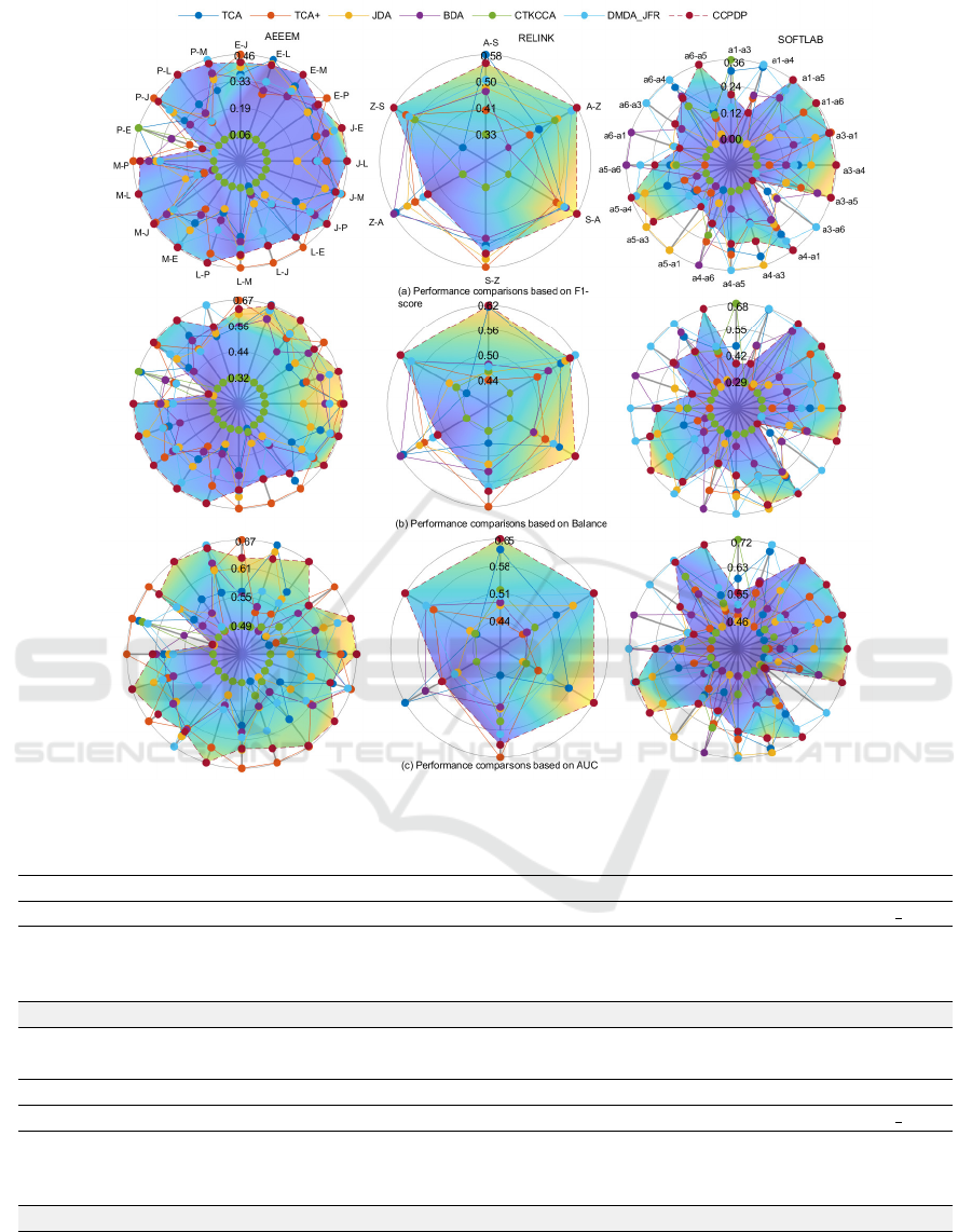
Figure 3: The figure displays nine different radar plots in three columns (each column represents a dataset). Each row
represents the performance of compared methods based on a metric.
Table 2: Win/Tie/Loss of CCPDP based on F1-score.
F1-score
TCA TCA+ JDA BDA CTKCCA DMDA JFR
AEEEM 17/0/3 11/0/9 18/0/2 18/0/2 19/0/1 17/1/2
RELINK 4/0/2 4/0/2 4/0/2 5/0/1 6/0/0 5/0/1
SOFTLAB 13/1/6 14/1/5 13/1/6 14/0/6 15/3/2 12/0/8
Total Win 34 (74%) 29 (63%) 35 (76%) 37 (80%) 40 (87%) 34 (74%)
Table 3: Win/Tie/Loss of CCPDP based on Balance.
Balance
TCA TCA+ JDA BDA CTKCCA DMDA JFR
AEEEM 17/0/3 14/0/6 19/0/1 19/0/1 19/0/1 17/0/3
RELINK 5/0/1 4/0/2 5/0/1 5/0/1 6/0/0 4/0/2
SOFTLAB 13/1/6 15/1/4 14/1/5 14/0/6 16/2/2 10/0/10
Total Win 35 (76%) 33 (72%) 38 (83%) 38 (83%) 41 (89%) 31 (67%)
Can a Simple Approach Perform Better for Cross-Project Defect Prediction?
333

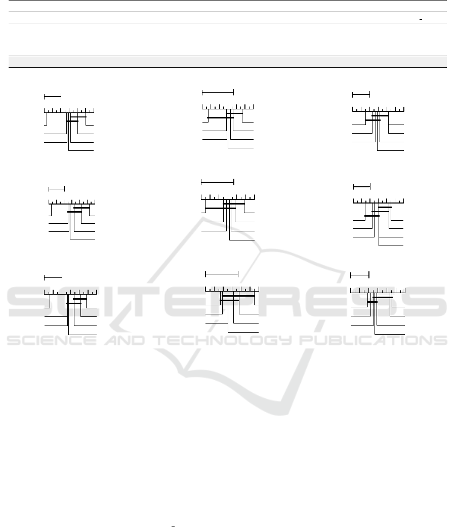
Table 4: Win/Tie/Loss of CCPDP based on AUC.
AUC
TCA TCA+ JDA BDA CTKCCA DMDA JFR
AEEEM 16/0/4 10/0/10 17/0/3 18/0/2 19/0/1 16/0/4
RELINK 5/0/1 5/0/1 6/0/0 5/0/1 6/0/0 6/0/0
SOFTLAB 14/1/5 17/0/3 15/1/4 15/0/5 17/1/2 11/0/9
Total Win 35 (76%) 32 (70%) 38 (83%) 38 (83%) 42 (91%) 33 (72%)
CD=2.01
7 6 5 4 3 2 1
CCPDP
TCA+
DMDA_JFR
TCA
BDA
JDA
CTKCCA
CD=3.68
7 6 5 4 3 2 1
CCPDP
DMDA_JFR
JDA
TCA
BDA
TCA+
CTKCCA
CD=2.01
7 6 5 4 3 2 1
CCPDP
DMDA_JFR
JDA
BDA
TCA
TCA+
CTKCCA
CD=2.01
7 6 5 4 3 2 1
CCPDP
TCA+
DMDA_JFR
BDA
JDA
TCA
CTKCCA
CD=3.68
7 6 5 4 3 2 1
CCPDP
DMDA_JFR
BDA
TCA
TCA+
JDA
CTKCCA
CD=2.01
7 6 5 4 3 2 1
DMDA_JFR
CCPDP
JDA
BDA
TCA
TCA+
CTKCCA
CD=2.01
7 6 5 4 3 2 1
CCPDP
TCA+
DMDA_JFR
TCA
JDA
BDA
CTKCCA
CD=3.68
7 6 5 4 3 2 1
CCPDP
DMDA_JFR
TCA
TCA+
BDA
CTKCCA
JDA
CD=2.01
7 6 5 4 3 2 1
CCPDP
DMDA_JFR
JDA
BDA
TCA
TCA+
CTKCCA
(g) AUC (AEEEM)
(h) AUC (RELINK)
(i) AUC (SOFTLAB)
(e) Balance (RELINK)
(f) Balance (SOFTLAB)
(d) Balance (AEEEM)
(a) F1-score (AEEEM)
(c) F1-score (SOFTLAB)
(b) F1-score (RELINK)
Figure 4: Statistic results using Nemenyi test for CCPDP and six other methods in terms of three performance metrics F1-score
(a,b,c), Balance (d,e,f) and AUC (g,h,i). Performances of methods connected by horizontal lines do not differ significantly.
We perform a significance test as mentioned
before. After rejecting the null hypothesis, the
ranking of the CCPDP and the compared methods are
then calculated. Fig. 4 illustrates the outcomes of the
Nemenyi test for F1-score, Balance and AUC metrics.
H
0
is rejected for all. Among nine tests (three for each
dataset), CCPDP achieves rank-1 (first) and rank-2
(second) in eight and one cases, respectively. Even
though CCPDP secured the second position in case of
SOFTLAB dataset for AUC metric, its performance
is not significantly different from DMDA JFR. Note
that, although CCPDP performs better in most of the
cases, many of the other methods do not significantly
differ with CCPDP. However, those methods require
high computational cost along with several tuning
parameters. Therefore, we can conclude that CCPDP
performs consistently better compared to existing
methods at a lower computational cost.
5 THREATS TO VALIDITY
It is shown that the utilization of correlation alignment
makes CCPDP consistently better than other methods
in three dataset. Due to the space limitation, we
only considered a single classifier random forest and
three popular metrics F1-score, Balance, and AUC
to evaluate the performance. Therefore, a change in
classifier such as decision tree, logistic regression and
metrics such as g-measure and MCC might result in
a different performance from the reported. Further,
we use datasets that are widely considered for CPDP
problem which includes 46 project-pairs. However,
this number may not generalize our findings. Finally,
though we have carefully implemented other methods
and followed the parameter settings according to the
suggestions of the respective paper, there might be a
chance of obtaining slightly different results for the
existing methods.
ENASE 2024 - 19th International Conference on Evaluation of Novel Approaches to Software Engineering
334

6 CONCLUSION
In this paper, we investigated a computationally
simple and parameter-free transfer learning based
method using CORAL for the cross-project defect
prediction problem which will provide a relief for
the users from the uncertainty of optimally tuning the
parameters and achieving the best results. This also
saves time and cost. Our CORAL based approach
CCPDP outperforms existing methods in most of the
cases. However, we observed that CORAL fails to
align source and target in some cases which can be
investigated in a future work.
ACKNOWLEDGEMENTS
This research is supported by the fellowship from ICT
Division, Ministry of Posts, Telecommunications and
Information Technology, Bangladesh.
REFERENCES
Akhter, S., Sajeeda, A., and Kabir, A. (2023). A distance-
based feature selection approach for software anomaly
detection. In ENASE, pages 149–157.
D’Ambros, M., Lanza, M., and Robbes, R. (2012).
Evaluating defect prediction approaches: a
benchmark and an extensive comparison. Empirical
software engineering, 17:531–577.
Herbold, S., Trautsch, A., and Grabowski, J. (2018). A
comparative study to benchmark cross-project defect
prediction approaches. In ICSE, pages 1063–1063.
Li, Z., Jing, X.-Y., Wu, F., Zhu, X., Xu, B., and
Ying, S. (2018). Cost-sensitive transfer kernel
canonical correlation analysis for heterogeneous
defect prediction. AUTOMAT SOFTW ENG, 25:201–
245.
Li, Z., Jing, X.-Y., Zhu, X., Zhang, H., Xu, B., and Ying,
S. (2019). Heterogeneous defect prediction with two-
stage ensemble learning. AUTOMAT SOFTW ENG,
26:599–651.
Liu, C., Yang, D., Xia, X., Yan, M., and Zhang, X.
(2019). A two-phase transfer learning model for
cross-project defect prediction. Information and
software technology, 107:125–136.
Long, M., Wang, J., Ding, G., Sun, J., and Yu,
P. S. (2013). Transfer feature learning with joint
distribution adaptation. In ICCV, pages 2200–2207.
Menzies, T., Caglayan, B., Kocaguneli, E., Krall, J., Peters,
F., and Turhan, B. (2012). The promise repository of
empirical software engineering data.
Menzies, T., Greenwald, J., and Frank, A. (2006). Data
mining static code attributes to learn defect predictors.
IEEE T SOFTWARE ENG, 33(1):2–13.
Menzies, T., Milton, Z., Turhan, B., Cukic, B., Jiang,
Y., and Bener, A. (2010). Defect prediction from
static code features: current results, limitations, new
approaches. AUTOMAT SOFTW ENG, 17:375–407.
Nam, J., Pan, S. J., and Kim, S. (2013). Transfer defect
learning. In 2013 35th ICSE, pages 382–391. IEEE.
Nemenyi, P. B. (1963). Distribution-free multiple
comparisons. Princeton university.
Niu, J., Li, Z., and Qi, C. (2021). Correlation
metric selection based correlation alignment for
cross-project defect prediction. In 2021 20th
IUCC/CIT/DSCI/SmartCNS, pages 490–495. IEEE.
Pal, S. and Sillitti, A. (2022). Cross-project defect
prediction: a literature review. IEEE access.
Pan, S. J., Tsang, I. W., Kwok, J. T., and Yang, Q. (2010).
Domain adaptation via transfer component analysis.
IEEE T NEURAL NETWOR, 22(2):199–210.
Peters, F., Menzies, T., and Marcus, A. (2013). Better cross
company defect prediction. In 2013 10th working
conference on MSR, pages 409–418. IEEE.
Qiu, S., Lu, L., and Jiang, S. (2019). Joint distribution
matching model for distribution–adaptation-based
cross-project defect prediction. IET software,
13(5):393–402.
Sharmin, S., Arefin, M. R., Abdullah-Al Wadud, M.,
Nower, N., and Shoyaib, M. (2015). Sal: An effective
method for software defect prediction. In 2015 18th
ICCIT, pages 184–189. IEEE.
Sun, B., Feng, J., and Saenko, K. (2017). Correlation
alignment for unsupervised domain adaptation.
Domain adaptation in computer vision applications,
pages 153–171.
Turhan, B., Menzies, T., Bener, A. B., and Di Stefano, J.
(2009). On the relative value of cross-company and
within-company data for defect prediction. Empirical
software engineering, 14:540–578.
Wei, P., Ke, Y., and Goh, C. K. (2018). Feature analysis
of marginalized stacked denoising autoenconder for
unsupervised domain adaptation. IEEE T NEUR NET
LEAR, 30(5):1321–1334.
Wu, R., Zhang, H., Kim, S., and Cheung, S.-C. (2011).
Relink: recovering links between bugs and changes.
In Proceedings of the 19th ACM SIGSOFT symposium
and the 13th ECFSE, pages 15–25.
Xu, Z., Pang, S., Zhang, T., Luo, X.-P., Liu, J., Tang,
Y.-T., Yu, X., and Xue, L. (2019). Cross project
defect prediction via balanced distribution adaptation
based transfer learning. J COMPUT SCI TECHNOL,
34:1039–1062.
Zhang, W., Zhang, X., Lan, L., and Luo, Z. (2020).
Maximum mean and covariance discrepancy for
unsupervised domain adaptation. Neural processing
letters, 51:347–366.
Zou, Q., Lu, L., Yang, Z., Gu, X., and Qiu,
S. (2021). Joint feature representation learning
and progressive distribution matching for cross-
project defect prediction. Information and software
technology, 137:106588.
Can a Simple Approach Perform Better for Cross-Project Defect Prediction?
335