X-GAN: Generative Adversarial Networks Training Guided with

Explainable Artiﬁcial Intelligence

Guilherme Botazzo Rozendo

1,5 a

, Alessandra Lumini

1 b

, Guilherme Freire Roberto

2 c

Tha

ına Aparecida Azevedo Tosta

3 d

, Marcelo Zanchetta do Nascimento

4 e

and Leandro Alves Neves

5 f

Department of Computer Science and Engineering (DISI) - University of Bologna, Cesena, Italy

Faculty of Engineering, University of Porto (FEUP), Porto, Portugal

Science and Technology Institute (ICT), Federal University of S

ao Paulo (UNIFESP), S

ao Jos

e dos Campos, Brazil

Faculty of Computer Science (FACOM), Federal University of Uberl

andia (UFU), Uberl

andia, Brazil

Department of Computer Science and Statistics (DCCE), S

ao Paulo State University, S

ao Jos

e do Rio Preto, Brazil

Keywords:

Generative Adversarial Networks, Explainable Artiﬁcial Intelligence, GAN Training.

Abstract:

Generative Adversarial Networks (GANs) create artiﬁcial images through adversary training between a gen-

erator (G) and a discriminator (D) network. This training is based on game theory and aims to reach an

equilibrium between the networks. However, this equilibrium is hardly achieved, and D tends to be more pow-

erful. This problem occurs because G is trained based on only a single value representing D’s prediction, and

only D has access to the image features. To address this issue, we introduce a new approach using Explainable

Artiﬁcial Intelligence (XAI) methods to guide the G training. Our strategy identiﬁes critical image features

learned by D and transfers this knowledge to G. We have modiﬁed the loss function to propagate a matrix

of XAI explanations instead of only a single error value. We show through quantitative analysis that our ap-

proach can enrich the training and promote improved quality and more variability in the artiﬁcial images. For

instance, it was possible to obtain an increase of up to 37.8% in the quality of the artiﬁcial images from the

MNIST dataset, with up to 4.94% more variability when compared to traditional methods.

1 INTRODUCTION

Generative adversarial networks (GANs) (Goodfel-

low et al., 2014) are generative models composed of

a pair of neural networks: the generator (G) and the

discriminator (D). G aims to learn the probability dis-

tribution function from a set of samples and synthe-

size new images following the learned function. D

receives original images and those synthesized by G

as input and tries to differentiate between them. Both

networks are trained at the same time with different

objectives. G tries to produce increasingly realistic

images to fool the discriminator and maximize classi-

https://orcid.org/0000-0002-4123-8264

https://orcid.org/0000-0003-0290-7354

https://orcid.org/0000-0001-5883-2983

https://orcid.org/0000-0002-9291-8892

https://orcid.org/0000-0003-3537-0178

https://orcid.org/0000-0001-8580-7054

ﬁcation error. D attempts to become increasingly bet-

ter at detecting which images are authentic and which

are artiﬁcial, minimizing classiﬁcation error. This an-

tagonistic training strategy is based on game theory.

It aims to reach an equilibrium point, the Nash equi-

librium, which corresponds to the situation in which

G produces images identical to the original ones, and

D can no longer differentiate the authentic from arti-

ﬁcial images (Trevisan de Souza et al., 2023).

However, training GANs is challenging due to is-

sues related to backpropagation, particularly in how

the G’s weights are updated. The backpropagation

process only shares D’s classiﬁcation results with G,

and as G receives random noise as input, it has no in-

formation about how the images’ features contributed

to classiﬁcation. Therefore, only D can access the rel-

evance of these features. Consequently, D tends to as-

sign higher scores to real images throughout the train-

ing, and G fails to fool D even after the model con-

674

Rozendo, G., Lumini, A., Roberto, G., Tosta, T., Zanchetta do Nascimento, M. and Neves, L.

X-GAN: Generative Adversarial Networks Training Guided with Explainable Artiﬁcial Intelligence.

DOI: 10.5220/0012618400003690

Paper published under CC license (CC BY-NC-ND 4.0)

In Proceedings of the 26th International Conference on Enterprise Information Systems (ICEIS 2024) - Volume 1, pages 674-681

ISBN: 978-989-758-692-7; ISSN: 2184-4992

verges (Wang et al., 2022; Trevisan de Souza et al.,

2023).

Studies in the literature usually aim to improve the

discriminator due to its crucial role in training (Ar-

jovsky et al., 2017; Gulrajani et al., 2017; Jolicoeur-

Martineau, 2018; Wang et al., 2021). However, there

has been a shift in focus in recent years towards im-

proving the training of the generator. The new ap-

proaches involve ﬁnding effective ways to transfer

the knowledge about the image features learned by

the discriminator to the generator (Wang et al., 2022;

Trevisan de Souza et al., 2023). One potential so-

lution is to combine GANs with explainable artiﬁ-

cial intelligence (XAI). XAI methods arose from the

need for more transparency and interpretability in the

decision-making process of deep learning algorithms.

It generates explanations illustrating which patterns a

model has learned or which parts of the input were

considered the most important for the model, thus

providing conditions for humans to understand why a

decision was made (Nielsen et al., 2022). On the other

hand, artiﬁcial neural networks simulate the function-

ing of the human brain, which includes the visual

cortex responsible for processing visual information.

These facts prompt whether XAI methods can pro-

vide relevant information to a GAN as they provide it

to humans.

We propose using XAI methods to identify the

most critical features of the input that the discrimi-

nator utilized to classify the images and feed this in-

formation into G. We use traditional architectures as a

basis and modify the loss function to propagate a ma-

trix instead of just an error value. This matrix derives

from the explanations generated by the XAI methods

and the discriminator error. Goodfellow et al. (Good-

fellow et al., 2014) use the forger versus police anal-

ogy to illustrate the training of GANs. In this analogy,

G plays the role of a forger who produces fake prod-

ucts, and D is a detective trying to identify whether

the products are original. Our method proposes ex-

panding the forger versus detective relationship to a

student versus teacher relationship. In the new anal-

ogy, G plays the role of a student who learns to repro-

duce works of art, and D is a teacher who evaluates

the work produced by the student, indicating where

the student has to focus to produce better art.

Therefore, this work presents a new way to train

GANs that includes XAI’s explanations in the back-

propagation algorithm to guide G’s training. We show

through experiments that our proposal not only im-

proves the quality of the images but also promotes an

increase in image variability. This research makes the

following signiﬁcant contributions: 1. An approach

that feeds G with substantial information concern-

ing the images’ features, increasing the quality of the

generated images; 2. The enrichment of D feedback

that promotes a greater variability in the generation

of artiﬁcial images, and; 3. A quantitative compar-

ison between the proposed model’s capabilities and

established architectures on commonly utilized image

datasets within specialized literature, such as MNIST

and CIFAR10.

2 RELATED WORK

One of the ﬁrst attempts at improving the training was

introducing the DCGAN, where the challenge was

creating a GAN architecture using convolutional lay-

ers. The strategies focused on changing the discrim-

inator to make it more stable. It included batch nor-

malization and leaky ReLU activations between inter-

mediate layers of the discriminator and the minimiza-

tion of the number of fully connected layers (Wang

et al., 2021). However, the DCGAN uses the orig-

inal Jensen-Shannon divergence as the loss function

(Goodfellow et al., 2014), which leads to training in-

stability.

WGAN (Arjovsky et al., 2017) is a technique that

enhances the training of GANs by replacing the tra-

ditional loss function with the Wasserstein distance.

The Wasserstein distance is a continuous measure

of the difference between probability distributions,

which helps to improve training stability. WGAN en-

forces the Lipschitz constraint on the discriminator by

using weight clipping. However, this technique can

lead to undesired side effects, such as vanishing or

exploding gradients, which may decrease the model’s

learning capacity. WGAN-GP (Gulrajani et al., 2017)

employs a gradient penalty term in the loss function

instead of weight clipping to address these issues.

This approach penalizes the norm of the gradient of

the discriminator concerning its input, thus helping

to maintain the Lipschitz constraint without weight

clipping. It is considered a more stable alternative to

weight clipping.

RAGAN (Jolicoeur-Martineau, 2018) is another

way to make the training more stable. It introduces

the relativistic discriminator, where instead of just

classifying whether an input is real or fake, it esti-

mates the probability that an authentic sample is more

realistic than a fake sample and vice versa. This rel-

ativistic approach improves the training stability and

quality of generated samples in speciﬁc scenarios. It

provides a more nuanced signal to the generator, al-

lowing it to understand better how to generate plausi-

ble samples not just on its own but also in relation to

the real data distribution.

X-GAN: Generative Adversarial Networks Training Guided with Explainable Artiﬁcial Intelligence

675

Newer techniques now focus on improving the

generator’s training rather than the discriminator. For

instance, the EqGAN-SA (Wang et al., 2022) is a

training technique that reduces the information imbal-

ance between D and G by enabling spatial awareness

of G and aligning it with D’s attention maps. The

method randomly samples heatmaps from the dis-

criminator using Grad-CAM and integrates them into

the feature maps of G via the spatial encoding layer.

Another strategy is GLeaD (Bai et al., 2023),

which introduces a new training paradigm to establish

a fairer game setting between G and D. The method

is based on the premise that D does not act as a player

but rather as a referee in the adversarial game. There-

fore, to balance the networks, the method introduces

a generator-leading task in which the discriminator

must extract features that G can decode to reconstruct

the input.

3 METHODOLOGY

Figure 1 shows an overview of the proposed model,

the X-GAN. The model uses architectures such as

DCGAN, WGAN-GP, and RAGAN as the basis for

G and D. Therefore, G receives a random signal vec-

tor z and outputs an image I

, and D classiﬁes authen-

tic I

and artiﬁcial images I

. The main novelty of

the proposed method is the inclusion of XAI expla-

nation (E) in the loss function to guide the training

of G, performing a new form of training called edu-

cational training. The new loss L

uses traditional

adversary losses (L

adv

) combined with the explana-

tions (E) to backpropagate important information to

the generator. This new training follows a student

versus professor-analogy, in which the professor (D)

teaches the learned features to the student (G).

XAI

adv

Figure 1: Schematic summary of the proposed model.

3.1 Models

As a basis for our method, we used the DCGAN,

WGAN-GP, and RAGAN models to deﬁne the archi-

tectures and loss functions L

adv

and L

adv

3.1.1 DCGAN

The DCGAN performs the traditional adversarial

training (Goodfellow et al., 2014), where a gener-

ator and a discriminator are trained simultaneously

through a min-max game. The loss for the discrimina-

tor was calculated through the binary cross-entropy:

DCGAN

= −

∑

i=1

log(D(x

)) + log(1 − D(z

)), (1)

where m is the number of real samples x, D(x

) is the

D’s output for the real sample x

, z

is a random noise

vector, and D(z

) is the D’s output for the generated

images G(z

For real samples, D tries to maximize the proba-

bility of assigning them a value close to 1. For arti-

ﬁcial samples, D aims to minimize the probability of

assigning a high value to them, i.e., tries to assign a

value close to zero.

The DCGAN generator’s loss considers D’s out-

put for the generated samples and tries to maximize

the probability of the discriminator assigning a value

close to 1 to the generated samples. It was deﬁned as:

DCGAN

= −

∑

i=1

log(1 − D(z

)). (2)

3.1.2 WGAN-GP

WGAN-GP uses the Wasserstein distance as a loss

function and a gradient penalty term to enforce the

Lipschitz continuity of the discriminator. The D’s ob-

jective is to approximate the Wasserstein distance be-

tween the actual and generated data distribution. The

Wasserstein distance is the difference between the ex-

pected values of the discriminator’s output for real

and generated samples:

= E

x∼P

data

[D(x)] − E

z∼P

noise

[D(G(z))]. (3)

The gradient penalty encourages the gradients of

the D’s output concerning the input to have a norm of

= λE

ˆx∼P

ˆx

[(∥∇

ˆx

D( ˆx)∥

− 1)

] (4)

where ˆx is a sample along a straight line between a

real sample and a generated sample, and λ is a hyper-

parameter that controls the strength of the penalty.

Thus, the adversarial loss for D was deﬁned as

the sum of the Wasserstein distance and the gradient

penalty:

W GAN−GP

= −L

+ L

, (5)

ICEIS 2024 - 26th International Conference on Enterprise Information Systems

676

and for G, as the negation the expected value of the

D’s output for generated samples:

W GAN−GP

= −E

z∼P

noise

[D(G(z))]. (6)

3.1.3 RAGAN

The RAGAN introduces the relativistic discriminator.

The primary idea is to compare the realism of real and

fake samples relative to each other instead of indepen-

dently. It can result in more stable training and better

convergence. The relative loss function is deﬁned as

follows:

rel

= −

x∼P

data

,z∼P

noise

[log(D(x) − D(G(z))]. (7)

The total loss for the discriminator was the sum

of the DCGAN loss and the relativistic discriminator

loss:

RAGAN

= L

DCGAN

+ L

rel

. (8)

Similar to the discriminator, the generator aims

to produce samples that are considered more realistic

than the average fake sample. Thus, the loss function

was deﬁned as:

RAGAN

= −

z∼P

noise

[log(1 − D(G(z))]−

x∼P

data

[log(D(x)].

(9)

3.2 XAI Methods

For this work, we have opted to use gradient-based

XAI techniques. The idea was to extract the most

important features from the discriminator gradients.

These methods rely on the gradients of the discrim-

inator’s output (logits or softmax probabilities) con-

cerning its input to construct explanations. These

techniques offer several beneﬁts, such as computa-

tional efﬁciency and the absence of restrictions on

speciﬁc architectures (Nielsen et al., 2022).

3.2.1 Saliency

The Saliency method (Simonyan et al., 2014) allowed

us to create explanations by calculating the gradients

of the D’s output concerning the input features. The

method takes an N-dimensional input x = {x

}

i=1

and

the associated C-dimensional output S(x) = {S

}

c=1

where C is the total number of classes, and calculates

the partial derivative of S(x) with respect to input x:

saliency

∂S

(x)

∂x

. (10)

The gradient represents how much the output

would change with a slight change in the input.

Thus, this method created maps highlighting regions

where a slight change in the input would signiﬁcantly

change the D’s predictions. In other words, it indi-

cates which features best represent an authentic im-

age.

3.2.2 InputXgrad

The InputXgrad (Shrikumar et al., 2017) generates the

explanations by calculating the elementwise multipli-

cation of gradients by the input:

InputXgrad

∂S

(x)

∂x

⊙ x (11)

We used this method because the elementwise

multiplication applies a model-independent ﬁlter,

in this case, the input, which reduces noise and

smoothens the explanations (Nielsen et al., 2022).

3.2.3 DeepLIFT

The DeepLIFT (Shrikumar et al., 2017) calculates the

difference between the activation of each neuron (or

feature) at a reference point and the input. This differ-

ence represents the contribution of each feature to the

overall output. We used the minimal activation, i.e.,

all zeros, as the reference point. The calculated differ-

ences were then distributed through the layers, con-

sidering the weights of the connections and the activa-

tion functions at each layer. The goal was to attribute

the contribution of each feature to different parts of

the network. DeepLIFT uses a backpropagation-like

adjustment to distribute the contributions. It aims to

fairly distribute the differences while accounting for

the role of each neuron in the network.

3.3 Loss Function

The main novelty of the proposed model is the new

form of training called educational training that fol-

lows a student versus professor analogy, in which the

professor (D) teaches the learned features to the stu-

dent (G). To perform this new way of training, we

included the XAI explanations in the G’s loss func-

tion as follows:

= L

adv

∗ E, (12)

in which ∗ is the multiplication operation, L

adv

the adversarial loss for the generator (Equation 2, 6,

or 9), and E is the XAI explanations generated with

Saliency, DeepLIFT, and InputXgrad, from the artiﬁ-

cial images.

X-GAN: Generative Adversarial Networks Training Guided with Explainable Artiﬁcial Intelligence

677

The gradient is a vector of real numbers that al-

lows us to determine the amount that must be adjusted

in each weight of G so that the loss function walks to-

wards minimization. Integrating E within the gradient

enables emphasis on areas corresponding to objects

of interest while dampening the inﬂuence of less rele-

vant regions. In the student versus professor analogy,

E corresponds to a test answer in which the professor

(D) informs the student (G) of his/her test score, in-

dicating where the error is, i.e., which features drawn

are close to reality and which are not similar to the

original images. Therefore, instead of propagating

just one value that indicates the error of D, we propa-

gate a matrix with relevant information for each pixel

in the image.

To propagate a matrix instead of a scalar, it is

necessary to perform an operation known as vector-

Jacobian Product, deﬁned as:

J ·⃗v, (13)

where J is the Jacobian matrix and⃗v is a multidimen-

sional vector of the same dimension as the explana-

tions E with 1 in all positions.

The Jacobian matrix indicates how the output

changes when a small amount of the input changes.

Thus, the proposed method deﬁnes the change that

each pixel of the artiﬁcial image causes in the predic-

tion of D. Moreover, the proposal also assigns greater

weights to the more relevant pixels.

3.4 Datasets

The MNIST dataset (LeCun et al., 1998), shown in

Figure 2, is a widely used collection of handwritten

digit images commonly employed for training vari-

ous image processing systems and machine learning

models. It consists of grayscale images of handwrit-

ten digits (0 through 9) centered within the images.

Each image is a 28 × 28 pixel square.

Figure 2: Examples from the MNIST dataset.

The CIFAR-10 dataset (Krizhevsky, 2009) is an-

other widely used benchmark dataset in computer vi-

sion and machine learning. It comprises 60,000 32 ×

32 color images in 10 different classes. Each image

belongs to the following classes: airplane, automo-

bile, bird, cat, deer, dog, frog, horse, ship, or truck.

Figure 3 shows examples from some classes from the

dataset (airplane, automobile, and cat).

Figure 3: Examples from the CIFAR10 dataset.

3.5 Performance Evaluation

3.5.1 Fr

echet Inception Distance

We applied the Fr

echet Inception Distance (FID) met-

ric (Heusel et al., 2017) to assess the quality of arti-

ﬁcial images quantitatively. This metric measures the

distance between the distributions of real and gener-

ated images. Therefore, lower FID scores indicate

higher similarity between the distributions, meaning

that the generated images closely resemble the origi-

nal ones.

The FID measures the similarity between two

multivariate Gaussian distributions, deﬁned by the

mean and covariance matrix of activation features ex-

tracted from Inception v3’s 2048th layer. Mathemati-

cally, The FID score is deﬁned by:

FID = ∥µ

− µ

∥

+ Tr(Σ

+ Σ

− 2(Σ

· Σ

)

0.5

), (14)

where µ

and µ

are the mean features of real and fake

images. Σ

and Σ

are the covariance matrices of real

and fake image features, and Tr(·) denotes the trace

of a matrix.

3.5.2 Inception Score

We also applied the Inception Score (IS) metric (Sal-

imans et al., 2016) to estimate the diversity of gener-

ated images. A higher IS suggests greater variety in

the assigned classes, although it does not necessarily

indicate a high degree of realism.

In the IS calculation, fake images were evalu-

ated based on the activations of the ﬁnal classiﬁca-

tion layer of a pre-trained Inception v3 model. This

model assigns a probability distribution to each image

over predeﬁned classes in the ImageNet dataset. Di-

verse images are expected to have probabilities spread

across multiple classes. The IS was calculated by tak-

ing the average entropy of all generated images and

computing its exponential value:

IS = exp(E

(p(y|x)||p(y))]), (15)

where p(y|x) is the probability of class y being as-

signed to the generated image x, p(y) is the marginal

probability of class y in the dataset, E

denotes

the expectation taken over all generated images,

(p(y|x)||p(y)) is the Kullback-Leibler divergence

between p(y|x) and p(y) and exp(·) represents the ex-

ponential function.

ICEIS 2024 - 26th International Conference on Enterprise Information Systems

678

3.6 Experiments Setup

We conducted this research through two experiments,

one in the MNIST and the other in the CIFAR10

dataset. We used the same GAN architecture for

both experiments, following the work of (Jolicoeur-

Martineau, 2018). We used a generator with ﬁve

transposed convolutional layers with batch normaliza-

tion, ReLU activation, and the Tanh function after the

last layer. For the discriminator, we used six convolu-

tional layers with BatchNorm and LeakyReLU. The

sigmoid activation function was used in DCGAN but

not in WGAN-GP and RAGAN.

Our models were trained for 100 epochs in batches

of size 32, with a z size 128. To ensure fair perfor-

mance evaluation, we ran each method ten times and

compared the simple average of the FID and IS met-

rics. We estimated these metrics using 50 thousand

images. For standardization purposes, we normalize

the explanations from all XAI methods to the range

[1,2].

3.7 Execution Environment

The proposed method was implemented using Python

3.9.16 and the Pytorch 1.13.1 API. The experiments

were performed on a computer with a 12th Generation

Intel

Core™i7-12700, 2.10GHz, NVIDIA

GeForce

RTX™3090 card, 64 GB of RAM and Windows op-

erating system with 64-bit architecture.

4 RESULTS AND DISCUSSION

Tables 1, 2, and 3 show the averaged FID and IS on

the MNIST dataset regarding the DCGAN, WGAN-

GP, and RAGAN-based architectures, respectively.

Table 1 shows that using the Saliency method with the

DCGAN architecture improved the quality of the arti-

ﬁcial images. XDCGAN (Saliency) produced images

of better quality, with an FID score around 3.72%

lower than DCGAN. In addition, the images gener-

ated with XDCGAN (Saliency) were more diverse, as

evidenced by an IS score of 2.1294, slightly higher

than the 2.1289 obtained with DCGAN.

Table 1: Averaged FID and IS scores on MNIST dataset

using DCGAN-based architectures.

FID IS

DCGAN 2.3428 2.1289

XDCGAN (Saliency) 2.2572 ↓ 2.1294 ↑

XDCGAN (DeepLIFT) 2.6792 ↑ 2.1239 ↓

XDCGAN (InputXgrad) 2.7468 ↑ 2.1168 ↓

In Table 2, it is veriﬁed that the proposed method

outperforms WGAN-GP signiﬁcantly. XWGAN-

GP (DeepLIFT) and XWGAN-GP (InputXgrad) pro-

duced images with an FID up to 37.8% lower than

those generated by WGAN-GP. Moreover, it is im-

portant to note that all XWGAN-GP methods have

increased the variability of the images obtained com-

pared to WGAN-GP. For instance, XWGAN-GP (In-

putXgrad) produced an IS value of 2.2822, approx-

imately 4.94% higher than the IS value provided by

WGAN-GP.

Table 2: Averaged FID and IS scores on MNIST dataset

using WGAN-GP-based architectures.

FID IS

WGAN-GP 11.0952 2.1721

XWGAN-GP (Saliency) 12.0221 ↑ 2.1724 ↑

XWGAN-GP (DeepLIFT) 7.5686 ↓ 2.2673 ↑

XWGAN-GP (InputXgrad) 7.6735 ↓ 2.2822 ↑

Considering the RAGAN architecture (Table 3),

the proposed method also provided relevant results.

The highlight was XRAGAN (Saliency), which im-

proved the quality and variability of artiﬁcial images.

With this combination, obtaining an FID of 15.79%

lower than RAGAN and an IS of 2.0041 was possi-

ble.

Table 3: Averaged FID and IS scores on MNIST dataset

using RAGAN-based architectures.

FID IS

RAGAN 33.8299 1.9831

XRAGAN (Saliency) 28.8780 ↓ 2.0041 ↑

XRAGAN (DeepLIFT) 33.5152 ↓ 1.9532 ↓

XRAGAN (InputXgrad) 31.1702 ↓ 1.9652 ↓

Tables 4, 5, and 6 show the results obtained from

the CIFAR10 dataset. Using the XAI methods with

the DCGAN architecture (Table 4), it was possible to

obtain a slight quality improvement in the artiﬁcial

images with the XDCGAN (Saliency) and XDCGAN

(DeepLIFT) methods. These methods provided FIDs

of 30.9560 and 30.8860, lower values compared to

DCGAN (FID = 31.0575). The XDCGAN (Saliency)

also increased the IS metric, 2.1724, against 2.1721

provided by DCGAN.

When considering the WGAN-GP architecture,

we did not achieve an increase in quality when gener-

ating images from the CIFAR10 dataset. Despite this,

it is possible to notice in Table 5 that in all XWGAN-

GP combinations, there was a slight increase in the

variability of the artiﬁcial images.

On the other hand, when considering the RA-

X-GAN: Generative Adversarial Networks Training Guided with Explainable Artiﬁcial Intelligence

679

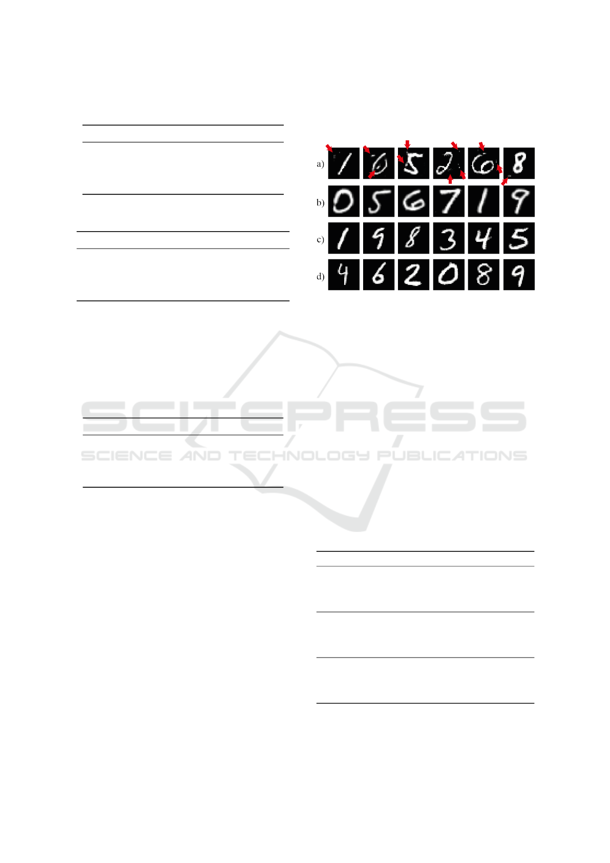
Table 4: Averaged FID and IS scores on CIFAR10 dataset

using DCGAN-based architectures.

FID IS

DCGAN 31.0575 6.7349

XDCGAN (Saliency) 30.9560 ↓ 6.7764 ↑

XDCGAN (DeepLIFT) 30.8860 ↓ 6.6785 ↓

XDCGAN (InputXgrad) 31.1186 ↑ 6.6900 ↓

Table 5: Averaged FID and IS scores on CIFAR10 dataset

using WGAN-GP-based architectures.

FID IS

WGAN-GP 33.9477 6.5254

XWGAN-GP (Saliency) 35.3156 ↑ 6.6791 ↑

XWGAN-GP (DeepLIFT) 34.4661 ↑ 6.6555 ↑

XWGAN-GP (InputXgrad) 35.1785 ↑ 6.5954 ↑

GAN architecture (Table 6), it was possible to ob-

tain an increase in the quality of artiﬁcial images with

all XRAGAN combinations, with emphasis on XRA-

GAN (DeepLIFT), which, in addition to promoting

increased quality, also generated images with more

variety compared to RAGAN.

Table 6: Averaged FID and IS scores on CIFAR10 dataset

using RAGAN-based architectures.

FID IS

RAGAN 32.2899 6.7158

XRAGAN (Saliency) 32.0886 ↓ 6.6762 ↓

XRAGAN (DeepLIFT) 32.0968 ↓ 6.7174 ↑

XRAGAN (InputXgrad) 31.4539 ↓ 6.6980 ↓

To illustrate the quantitative results, we present

in Figure 4 some examples of artiﬁcial images gen-

erated by WGAN-GP and XWGAN-GP variants on

the MNIST dataset. It is worth noting that images

produced by WGAN-GP have some defects, such as

noise and artifacts. These defects are highlighted with

red arrows in Figure 4a. Meanwhile, the images gen-

erated by XWGAN-GP (Saliency) have a blur effect

(Figure 4b). Although the blur effect is undesirable

in generating artiﬁcial images, this indicates that in-

formation was included in the generator training. It is

also possible to note that this combination eliminated

the noise and artifacts.

On the other hand, the images created by

XWGAN-GP (DeepLIFT) and XWGAN-GP (In-

putXgrad) (Figures 4c and 4d) are crisp and noise-

free, nearly indistinguishable from the images in the

original dataset (as shown in Figure 2). Therefore,

the difference in FID presented in Table 2 is due

to these factors. These combinations resulted in the

most signiﬁcant reduction in FID, with XWGAN-

GP (DeepLIFT) showing a decrease of 37.8% and

XWGAN-GP (InputXgrad) showing a decrease of

30.9% in comparison to XGAN-GP.

Figure 4: Examples of artiﬁcial images generated by

WGAN-GP (a), and by XWGAN-GP with the Saliency (b),

DeepLIFT (c) and InputXgrad (d) methods.

Table 7 shows the average time, in seconds, that

each method took to execute each epoch, consid-

ering an execution of 100 epochs and the conﬁgu-

rations mentioned in section 3.7. It is possible to

note that the proposed method does not cause a sub-

stantial increase in the processing time of GANs.

Considering, for example, the case that provided the

most signiﬁcant difference in FID, i.e., XWGAN-GP

(DeepLIFT) in the MNIST dataset, the time differ-

ence compared to WGAN-GP was only 21 seconds

more per epoch. Thus, the proposed method provided

a 37.8% reduction in FID with an increase of only

15.79% in processing time. It is also important to

note that XWGAN-GP (InputXgrad), which provided

a 30.9% decrease in the FID of the MNIST dataset,

only caused a 4.51% increase in processing time.

Table 7: Average time per epoch in seconds.

MNIST CIFAR10

DCGAN 70 60

XDCGAN (Saliency) 80 (14.29%) 65 (8.33%)

XDCGAN (DeepLIFT) 96 (37.14%) 80 (33.33%)

XDCGAN (InputXgrad) 82 (17.14%) 67 (11.67%)

WGAN-GP 133 108

XWGAN-GP (Saliency) 138 (3.76%) 118 (9.29%)

XWGAN-GP (DeepLIFT) 154 (15.79%) 131 (21.30%)

XWGAN-GP (InputXgrad) 139 (4.51%) 117 (8.33%)

RAGAN 73 62

XRAGAN (Saliency) 84 (15.07%) 72 (16.13%)

XRAGAN (DeepLIFT) 98 (34.25%) 83 (33.87%)

XRAGAN (InputXgrad) 85 (16.44%) 70 (12.90%)

ICEIS 2024 - 26th International Conference on Enterprise Information Systems

680

5 CONCLUSIONS

In this work, we present a new way to train GANs

using XAI explanations to guide the training of the

generator. The idea was to extract the most crit-

ical features from the images and provide them to

the generator during the training. Through quantita-

tive experiments, we demonstrate that the proposed

method improved the quality of the generated images.

It was possible to obtain an increase of up to 37.8%

in the quality of the artiﬁcial images from the MNIST

dataset, with up to 4.94% more variability when com-

pared to traditional methods. We show that this sig-

niﬁcant difference was achieved with little increase

in processing time. For example, it was possible to

obtain a 30.9% decrease in FID with just a 4.51% in-

crease in processing time. Although it was not pos-

sible to select a speciﬁc combination of methods for

all datasets, it is possible to note that the proposed

method always improved image quality or variability.

In future works, we intend to conduct new tests

with different combinations of GAN models and dif-

ferent ways to extract information from the images.

We believe that the improvement of the generator

training is a ﬁeld that is still little explored, with much

room for improvement. We also intend to analyze

how stable the proposed method is compared to tra-

ditional methods. Finally, we intend to investigate

the relevance of artiﬁcial images in data augmentation

problems.

ACKNOWLEDGEMENTS

This research was funded in part by the: Coordenac¸

de Aperfeic¸oamento de Pessoal de N

ıvel Superior

- Brasil (CAPES) – Finance Code 001; National

Council for Scientiﬁc and Technological Develop-

ment CNPq (#313643/2021-0 and #311404/2021-9);

the State of Minas Gerais Research Foundation -

FAPEMIG (Grant #APQ-00578-18); S

ao Paulo Re-

search Foundation - FAPESP (Grant #2022/03020-1).

REFERENCES

Arjovsky, M., Chintala, S., and Bottou, L. (2017). Wasser-

stein generative adversarial networks. In Interna-

tional conference on machine learning, pages 214–

223. PMLR.

Bai, Q., Yang, C., Xu, Y., Liu, X., Yang, Y., and Shen,

Y. (2023). Glead: Improving gans with a generator-

leading task. In Proceedings of the IEEE/CVF Con-

ference on Computer Vision and Pattern Recognition,

pages 12094–12104.

Goodfellow, I. J., Pouget-Abadie, J., Mirza, M., Xu, B.,

Warde-Farley, D., Ozair, S., Courville, A., and Ben-

gio, Y. (2014). Generative adversarial nets. In Pro-

ceedings of the 27th International Conference on Neu-

ral Information Processing Systems-Volume 2, pages

2672–2680.

Gulrajani, I., Ahmed, F., Arjovsky, M., Dumoulin, V., and

Courville, A. (2017). Improved training of wasser-

stein gans. In Proceedings of the 31st International

Conference on Neural Information Processing Sys-

tems, pages 5769–5779.

Heusel, M., Ramsauer, H., Unterthiner, T., Nessler, B., and

Hochreiter, S. (2017). Gans trained by a two time-

scale update rule converge to a local nash equilibrium.

In Guyon, I., Luxburg, U. V., Bengio, S., Wallach, H.,

Fergus, R., Vishwanathan, S., and Garnett, R., editors,

Advances in Neural Information Processing Systems,

volume 30. Curran Associates, Inc.

Jolicoeur-Martineau, A. (2018). The relativistic discrimina-

tor: a key element missing from standard gan. In In-

ternational Conference on Learning Representations.

Krizhevsky, A. (2009). Learning multiple layers of fea-

tures from tiny images. Technical report, University

of Toronto.

LeCun, Y., Bottou, L., Bengio, Y., and Haffner, P. (1998).

Gradient-based learning applied to document recogni-

tion. Proceedings of the IEEE, 86(11):2278–2324.

Nielsen, I. E., Dera, D., Rasool, G., Ramachandran, R. P.,

and Bouaynaya, N. C. (2022). Robust explainability:

A tutorial on gradient-based attribution methods for

deep neural networks. IEEE Signal Processing Mag-

azine, 39(4):73–84.

Salimans, T., Goodfellow, I., Zaremba, W., Cheung, V.,

Radford, A., Chen, X., and Chen, X. (2016). Im-

proved techniques for training gans. In Lee, D.,

Sugiyama, M., Luxburg, U., Guyon, I., and Garnett,

R., editors, Advances in Neural Information Process-

ing Systems, volume 29. Curran Associates, Inc.

Shrikumar, A., Greenside, P., and Kundaje, A. (2017).

Learning important features through propagating ac-

tivation differences. In International conference on

machine learning, pages 3145–3153. PMLR.

Simonyan, K., Vedaldi, A., and Zisserman, A. (2014). Deep

inside convolutional networks: visualising image clas-

siﬁcation models and saliency maps. In Proceedings

of the International Conference on Learning Repre-

sentations (ICLR), pages 1–8. ICLR.

Trevisan de Souza, V. L., Marques, B. A. D., Batagelo,

H. C., and Gois, J. P. (2023). A review on generative

adversarial networks for image generation. Comput-

ers & Graphics, 114:13–25.

Wang, J., Yang, C., Xu, Y., Shen, Y., Li, H., and Zhou,

B. (2022). Improving gan equilibrium by raising spa-

tial awareness. In Proceedings of the IEEE/CVF Con-

ference on Computer Vision and Pattern Recognition,

pages 11285–11293.

Wang, Z., She, Q., and Ward, T. E. (2021). Generative

adversarial networks in computer vision: A survey

and taxonomy. ACM Computing Surveys (CSUR),

54(2):1–38.

X-GAN: Generative Adversarial Networks Training Guided with Explainable Artiﬁcial Intelligence

681