Unsupervised Anomaly Detection in Continuous Integration Pipelines
Daniel Gerber
1
, Lukas Meitz
2
, Lukas Rosenbauer
1
and J
¨
org H
¨
ahner
3
1
BSH Hausger
¨
ate GmbH, Im Gewerbepark B10, 93059 Regensburg, Germany
2
Technische Hochschule Augsburg, Fakult
¨
at Informatik, An der Hochschule 1, 86161 Augsburg, Germany
3
Universit
¨
at Augsburg, Lehrstuhl f
¨
ur Organic Computing, Am Technologiezentrum 8, 86159 Augsburg, Germany
Keywords:
Software Testing, Integration Testing, Performance Data, Machine Learning, Unsupervised Learning,
Anomaly Detection.
Abstract:
Modern embedded systems comprise more and more software. This yields novel challenges in development
and quality assurance. Complex software interactions may lead to serious performance issues that can have a
crucial economic impact if they are not resolved during development. Henceforth, we decided to develop and
evaluate a machine learning-based approach to identify performance issues. Our experiments using real-world
data show the applicability of our methodology and outline the value of an integration into modern software
processes such as continuous integration.
1 INTRODUCTION
Continuous integration (CI) (Fowler, 2006) is a
paradigm in computer science that provides a more
automatic approach to develop software components.
It refers to the practice of frequently integrating
changes into a common repository. This series of
steps is called a pipeline, which has a new software
version as its output (Red Hat, Inc., 2022). Frequently
executed runs of the CI pipeline, e.g., each night,
are improving the overall quality (Strandberg et al.,
2022). Automatic testing is a vital part of CI systems,
typically reflecting test levels, e.g., unit tests, inte-
gration tests, or system tests (Jorgensen, 2013). An-
other aspect is performance monitoring, which com-
plements mere testing efforts. During frequent CI
runs, a vast amount of performance data is generated,
such as CPU utilization, memory consumption, and
system pressure. To complement directly failing test
cases, a performance analysis can provide additional
information on potential bugs in the software (Hrusto
et al., 2022).
In large CI pipelines, many different software
components can be managed in parallel. For exam-
ple, depending on the different systems and variants
of a embedded systems manufacturer, various system
platforms can be targeted at the same time, as well.
This forms a multitude of systems, components, test-
ing situations, and their corresponding performance
data, which is to be analyzed ideally within a short
time span. Typically, within the time span of only one
day, checking data, taking informed decisions and act-
ing accordingly is often too much to be handled solely
by humans. Machine learning (ML) approaches, such
as anomaly detection, can provide a form of automa-
tion For example a potential ML system might raise
a flag and point developers to the latest build, in case
something unusual occurred in the latest run. To im-
plement such a system, the task of detecting mean-
ingful anomalies (helpful for developers and test en-
gineers) based on performance data in the CI pipeline
is to be solved.
In this paper, such a detection system is developed
and analyzed for its applicability and verified on the
testing infrastructure (as part of the CI pipeline) of
a consumer electronics manufacturer. In this infras-
tructure, different system platforms containing a con-
tainerized operating system, whose performance data
is recorded and automatically analyzed by means of
anomaly detection. The approach is targeting the a
priori unknown by learning what is normal behaviour
of the different system or container variables. This al-
lows to raise a flag if an unusual high anomaly scores
occur during a CI run. Additionally, the defined data
structure enables a systematic statistics on used sys-
tem resources, which can be used to define criteria for
system health. In order to restrict the search area in
the source code the overall approach is differentiating
336
Gerber, D., Meitz, L., Rosenbauer, L. and Hähner, J.
Unsupervised Anomaly Detection in Continuous Integration Pipelines.
DOI: 10.5220/0012618500003687
Paper published under CC license (CC BY-NC-ND 4.0)
In Proceedings of the 19th International Conference on Evaluation of Novel Approaches to Software Engineering (ENASE 2024), pages 336-343
ISBN: 978-989-758-696-5; ISSN: 2184-4895
Proceedings Copyright © 2024 by SCITEPRESS – Science and Technology Publications, Lda.

between individual system and containers variables,
which extends the usual test failure criteria by further
insights on the performance data recorded during test-
ing. In terms of traceability, the computed individual
anomaly scores allow a potential identification of the
underlying root causes:
• By taking into account which parts of the different
software components were changed compared to
previous commits.
• By having an indicator on which variables and
their associated software containers behave not as
expected. Each software service typically runs in
an independent container. If this particular con-
tainer behaves not within the expected ranges, it
can point towards an issue.
The rest of the paper is organized in the following
way: The related work section (Section 2) introduces
various touch points from research with this paper.
Afterwards (Section 3), the chosen approach to the
problem is outlined in terms of the related data and
algorithms in use. The outlined approaches are then
evaluated in terms of two experiment types (Section
4). The last section (Section 5) concludes this work
by summarizing and providing an outlook on future
research.
2 RELATED WORK
We are not the first to approach anomaly detection
based on performance data: In the area of qual-
ity assurance for software projects, Strandberg et al.
(Strandberg et al., 2022) deal with high-level test
management based on requirements, e.g., response
times of requests of a web service. Another approach
can be found on the test management layer. For ex-
ample, Capizzi et al. are working with different cri-
teria (lines of code, failed tests, issues in review, and
more) to judge whether to release or not to release a
software (Capizzi et al., 2020). Additionally, Hrusto
et al. are targeting the monitoring of performance
metrics in DevOps aspects of a micro-service sys-
tem (Hrusto et al., 2022). Cherkasova et al. are ob-
serving CPU-load profiles in an enterprise applica-
tion of a client-server architecture (Cherkasova et al.,
2009). Additionally, Atzberger et al. and Fawzy et
al. proposed log-based anomaly detection in CI/CD
pipelines (Atzberger. et al., 2023; Hany Fawzy et al.,
2023).
More general papers on anomaly detection are
giving additional insights into critical thinking around
the topic: Sehili et al. (El Amine Sehili and Zhang,
2023) state that papers in general often use F-score
Figure 1: Simplified schematic overview of the testing part
of the CI pipeline depicted in terms of flow of code and
collected performance data through the infrastructure.
to evaluate point anomaly events. One targeted type
of anomalies are memory leaks. Due to short test-
ing times and due to only subtle changes in the corre-
sponding memory-representing variables, a detection
performance indicator, such as F-Score, might not be
a sufficient discriminator for the selection of an algo-
rithm. In our experiments a more sophisticated way
is introduced, that consists of evaluating these algo-
rithms by a procedure from communication engineer-
ing, i.e., defining a metric targeting sensitivity.
When considering the previously mentioned per-
formance data as multivariate time series, the evalua-
tion of Garg et al. showed specifically the usefulness
of a simple univariate Autoencoder model (per vari-
able) to the problem of anomaly detection compared
to more sophisticated approaches (Garg et al., 2021).
In addition, Wu et al. (Wu and Keogh, 2021)
questioned the narrative that deep learning-based al-
gorithms are always the type of model to use and that
in many cases well established methods can result in
comparative results. To address this, we use three
different categories of anomaly detection algorithms
in our evaluations – a statistics-based, a classic ML-
based, and a Neural Network-based algorithm.
3 APPROACH
In this section, the underlying CI infrastructure, the
dataset definition, and the multivariate approach to
anomaly detection is outlined and explained.
3.1 Infrastructure
The software development infrastructure of the
household appliance manufacturer BSH Hausger
¨
ate
GmbH serves as a study object for this paper (BSH
Group, 2022). It is centered around the CI prin-
ciple. The CI pipeline employed by the embedded
Unsupervised Anomaly Detection in Continuous Integration Pipelines
337

software development is running on Jenkins servers
(Kawaguchi, 2011) on a nightly basis. As part of ev-
ery CI run, extensive automatic testing is conducted
to detect potential bugs or errors.
Figure 1 depicts a typical scenario, where a new
release candidate (code) is in the testing phase of a
CI cycle. During testing, the performance data is
recorded, which is stored on the company’s servers
and later-on analyzed for the decision making of the
actual software release. The device under test (DuT)
is an embedded Linux platform, on which the release-
candidate code is flashed and is running on a physical
hardware inside a testing rack.
One group of integration tests are the so-called
electronic component tests. These tests comprise sce-
narios that execute the communication of different
hardware units, or system boot up sequences. Dur-
ing testing, critical bugs might directly fail dedicated
tests. However, the goal of this research project is to
aim for more subtle problems, e.g., memory leaks, un-
usual behaviour of different variables, or unusual test
time prolongation.
The underlying assumption on this kind of analy-
sis is that the actual feature or requirement that is re-
flected by a certain test stays relatively constant com-
pared to changes in the actual source code, which
might contain errors or bugs that could lead to anoma-
lies that are detectable in the performance data it-
self. For example the so-called startup-time test stays
mostly the same over time, although a lot of different
commits are pushed into the version control system
within a year of development. This forms the founda-
tion for subsequent considerations.
3.2 Datasets
Three datasets are considered for the experiments:
A real-world test case dataset, an artificial Gaussian
random walk dataset, and an artificial noise dataset.
In general, the datasets are represented by a three-
dimensional array X, defined by
H × J × K = {(i, j, k)|i ∈ H , j ∈ J , k ∈ K }. (1)
The first dimension H = {0, 1, . . . , I − 1} describes
the meta-time index (i.e., the respective CI run), the
second dimension J = {0, 1, . . . , J − 1} the variable
index, and the third dimension K = {0, 1, . . . , K − 1}
the discrete time base of each variable. The number
of elements in the respective dimension are thereby
denoted as I, J, and K.
The real-world data is a representation of one spe-
cific test case (TC), that runs in the CI infrastructure.
Let X
TC
∈ R
I×J×K
represent one specific TC from I
CI runs, with J performance variables. K represents
thereby the maximum sequence length of all consid-
ered variables. In case variables are shorter than K,
they are padded by zero values to match the required
sequence length.
The first artificial dataset is the Noise dataset. It is
mimicking the same shape as the real-world counter-
part to provide a similar data complexity in terms of
dimensions. Without any presumptions on the data
apart from the shape, let X
N
∈ R
I×J×K
, whose en-
tries are drawn from a normal distribution X
i, j,k
∼
N (0, 1). Therefore, the Noise dataset contains no in-
herent trend in the data.
The second artificial dataset is the Gaussian ran-
dom walk (RW) dataset. It extends the previously in-
troduced noise dataset by RW sequences that repre-
sent a signal form, which is closer to the real-world
performance data due to the introduced trend in the
data. Consider J RW sequences of length K, that are
defined by X
k+1
= X
k
+Y , with Y ∼ N (0, 1), and k =
0, 1, . . . , K − 1. Let X
c
∈ R
I×J×K
, alongside the first
dimension of X
c
, a number of I copies of the J initial
RW sequences are contained in this array. By com-
bining X
c
and X
N
, we end up with X
RW
∈ R
I×J×K
,
defined by X
RW
= X
c
+ X
N
. The three datasets X
N
,
X
RW
, X
TC
are used as the basis of the subsequent ex-
periments.
3.3 Multivariate Schema
The main goal of anomaly detection is to identify the
respective CI run that appears anomalous compared to
other ones, which are deemed normal. Subsequently,
we aim at a deeper explainability in terms of the dif-
ferent individual variables in the datasets. Therefore,
our approach proposes an independent processing of
the variables, which supports also the scalability to an
arbitrary number of variables. Figure 2 provides an
overview on the proposed schema.
The dataset array X ∈ R
I×J×K
is split into its in-
dividual variables (also referred to as channels) X
j
∈
R
I×K
. The separation in channels helps to cope with
different value ranges, e.g., two orders of magnitude
in terms of CPU or more than six orders of magni-
tude in terms of memory-based variables. X
j
is nor-
malized according to its maximum value
e
X
j
=
X
j
max X
j
,
with
e
X
j
∈ R
I×K
. An anomaly detection (AD) algo-
rithm is applied to the normalized data of one channel
and is setup in such a way that it provides a continu-
ous anomaly score, which is generically represented
by function AD: R
I×K
→ R
I
. Respectively, the indi-
vidual anomaly score S
j
∈ R
I
of one channel is cal-
culated by
S
j
= AD(
e
X
j
). (2)
ENASE 2024 - 19th International Conference on Evaluation of Novel Approaches to Software Engineering
338

Figure 2: Multivariate anomaly detection (AD) schema.
The joint anomaly score S ∈ R
I
can be calculated over
the individual anomaly scores S
j
by
S =
∑
j
|
S
j
− µ
i
1
I
σ
i
|, (3)
where 1
I
= (1, 1, . . . , 1)
⊺
∈ R
I
. The joint anomaly
score S points us to the CI run that shows unusual
behavior, whereas the individual anomaly score S
j
shows us which variables deviate from normal behav-
ior in this particular CI run.
3.4 Algorithms
Starting by Equation 2, we ought to explain the
anomaly detection function AD in this section. Three
different types of algorithms are employed on the
given datasets: A statistical one, a classic ML method,
and a method based on neural networks.
3.4.1 Z-Score
As a comparable reference method from the family of
statistics-based methods, z-scores (Huck et al., 1986)
are employed as a simple method for anomaly detec-
tion inside the aforementioned schema.
e
X
k
is a single
normalized vector of length K from matrix
e
X
j
repre-
senting one time series of a single variable. µ
k
and σ
k
are mean and standard deviation that are operating on
dimension K for calculating the z-score. µ
k
and σ
k
are estimated on all I time series of
e
X
j
. The anomaly
score S
k
∈ R is calculated by
S
k
=
∑
k
|
e
X
k
− µ
k
1
K
σ
k
| (4)
for each row in
e
X
j
and 1
K
= (1, 1, . . . , 1)
⊺
∈ R
K
. The
anomaly score S
j
comprises all I z-scores S
k
after the
operation.
3.4.2 Isolation Forest
The tree-based isolation forest algorithm for anomaly
detection is used for comparison. Isolation forest
was introduced as a fast performing classical ma-
chine learning algorithm with multivariate capabili-
ties that can be trained on normally operating data
only (Liu et al., 2008). The isolation forest was cho-
sen as an additional type of algorithm, because of its
high-dimensional capabilities and solid performance
in other application domains. Especially in multivari-
ate time series applications this algorithm has suc-
cessfully been used, for example in detection of net-
work traffic anomalies (Tao et al., 2018) or user log
anomalies (Yang et al., 2023).
It works by building an ensemble of trees for par-
titioning of the training data (Schmidl et al., 2022).
This is achieved by randomly selecting features and
values for the partitioning, that will go on until each
sample in the training data is isolated by a tree. For
the detection of anomalies, the size of the trees needed
for isolation is important, as anomalies will be eas-
ier to separate from normal data points and therefore
need less decisions. Each channel j of the recorded
data is considered by a dedicated isolation forest
model with 100 estimators delivering S
j
in the exper-
iments.
3.4.3 Autoencoder
Initially published by Bourlard et al. (Bourlard and
Kamp, 1988), the neural-network based anomaly de-
tection is introduced – an Autoencoder model. It
has been successfully used in similar application do-
mains, like Torabi et al. detecting cyber attacks over
network traffic of cloud computing services (Torabi
et al., 2023). Or in Provotar et al. (Provotar et al.,
2019), where an Autoencoder model detected rare
sound events in time series data.
Autoencoders work by learning the representation
of training data through a bottleneck, where input data
is reconstructed from a compressed latent space. The
difference between input and output of an Autoen-
coder can be used as a metric, deemed reconstruction
error. The absolute of this error is used as an anomaly
score, based on the hypothesis that anomalous data is
reconstructed less effectively than normal data (Saku-
rada and Yairi, 2014).
Similar as described in Provotar et al. (Provotar
et al., 2019), we employ a neural network model to
the time series data. The data for each channel is
normalized and for each channel a separate Autoen-
Unsupervised Anomaly Detection in Continuous Integration Pipelines
339

coder model is employed. For this evaluation, a fully-
connected neural network with two layers of 128 neu-
rons (for encoder and decoder separately) and recti-
fied linear units has been used as the Autoencoder ar-
chitecture. The training process is performed by sam-
pling batches of time series from the input data
e
X
j
and is minimizing the reconstruction error on the net-
work’s outputs. The reconstruction error is calculated
by a mean squared error (MSE) criterion. This pro-
cess forms an inner representation described as the
Autoencoder’s latent space. Afterwards, the trained
model is applied to all input data rows for a final as-
sessment of the I anomaly scores S
j
for the j-th vari-
able channel.
4 EXPERIMENTS
The experiments’ strategy follows the base idea of
evaluating and fine-tuning the algorithms on two ar-
tificial datasets and apply them to real-world data,
where we do not have labels at hand. These experi-
ment groups are described in the following.
4.1 Artificial Anomaly Data
Experiments
The artificial anomaly data experiments contain gen-
erated anomalies that are added onto the two artificial
datasets – noise data X
N
and random walk data X
RW
.
We deem these controlled experiments, because by in-
troducing artificial anomalies onto the base data, the
indices for CI runs and variables are known a priori.
The three algorithms are compared against each other
on both datasets.
One of the presumptions of the overall task is to
find memory leaks as soon as possible in the devel-
opment process. Especially, static leaks can be prob-
lematic. They can be characterized by an accumu-
lation of memory consumption due to not appropri-
ately deallocating objects (Jung et al., 2014). One
way of modeling an artificial static memory leak on
the performance data is to add a linear function on a
memory-representing variable channel. For the sake
of simplicity, we randomly chose a variable regardless
of representing a memory-based variable or not. This
procedure represents a rise or decline of a variable
during testing. The steepness m is chosen to m =
h
K
,
which ensures the artificial anomaly to not exceed a
maximum height of h over the total time of K sam-
ples of the variable.
The maximum height is varied during the ex-
periments, i.e., h ∈ {.5, 1, 1.5, 2, 2.5, 3, 3.5, 4, 4.5, 5}.
Overall, the maximum heights are considered to
be rather small compared to the amplitudes deter-
mined by the normal distribution with σ
2
N
= 1 of the
noise floor. Due to the relatively short testing times
and a low accumulation of changes in the memory-
representing variables, the amplitudes of anomalies
are rather subtle, which emphasises the usefulness of
a measure based on sensitivity rather than a simple
F-Score.
Inspired by an approach from signal processing,
the minimal detectable signal (MDS) (Grigorakis,
1997) serves as a role model for the experiments with
artificial data. MDS is basically adjusting the signal-
to-noise ratio (SNR) of an input signal to a detection
unit, e.g., a radar or sonar detector unit. The SNR is
lowered until no more useful output signal can be de-
tected, which is a way to measure the sensitivity of
the detection unit.
Figure 3 shows an overview on the artificial exper-
iment. For the base data, noise data X
N
and random
walk data X
RW
come into operation. The experiment
is setup in such a way that for each time the exper-
iment is ran only one anomaly is added on one vari-
able. In order to measure the performance, a detection
metric is employed, which is deemed detection ratio
d
r
∈ R and in the following and defined by
d
r
:=

M
1
M
2
, i
t
= i
p
∧ j
t
= j
p
0, i
t
̸= i
p
∨ j
t
̸= j
p
(5)
The algorithms deliver a continuous anomaly
score for each CI run. If the detected CI run in-
dex i
p
of the first maximum of the anomaly score
is not matching with the true CI run index i
t
from
the anomaly generator and at the same time true vari-
able index j
t
is not matching with the predicted vari-
able index j
p
, than the detection ratio is set to zero
(d
r
= 0). If the detected indexes are matching, than
the ratio in Equation 5 is calculated out of the first
maximum value M
1
to the second maximum value
M
2
of the anomaly score. The metric indicates the
distance from the true maximum to the other values,
which allows a careful evaluation of the detection per-
formance.
As a statistical test, we employ Wilcoxon test
(Conover, 1971), following (Dem
ˇ
sar, 2006) for com-
paring classifiers. The null hypothesis H
0,12
: ˜x
1
≤ ˜x
2
with ˜x
1
= med
∀h
d
r1
, respectively. Table 1 shows the
p-values for the noise dataset and Table 2 for the ran-
dom walk dataset of the Wilcoxon tests, where the
row (e.g., 1) and columns (e.g., 2) are relating to the
null hypothesis (i.e., H
0,12
). The values in the lower
triangular of both tables are significantly low, which
indicates to reject the null hypothesis in those row-
column combinations. For example, row 3 indicates
the Autoencoder model to perform better than z-score
as well as isolation forest.
ENASE 2024 - 19th International Conference on Evaluation of Novel Approaches to Software Engineering
340

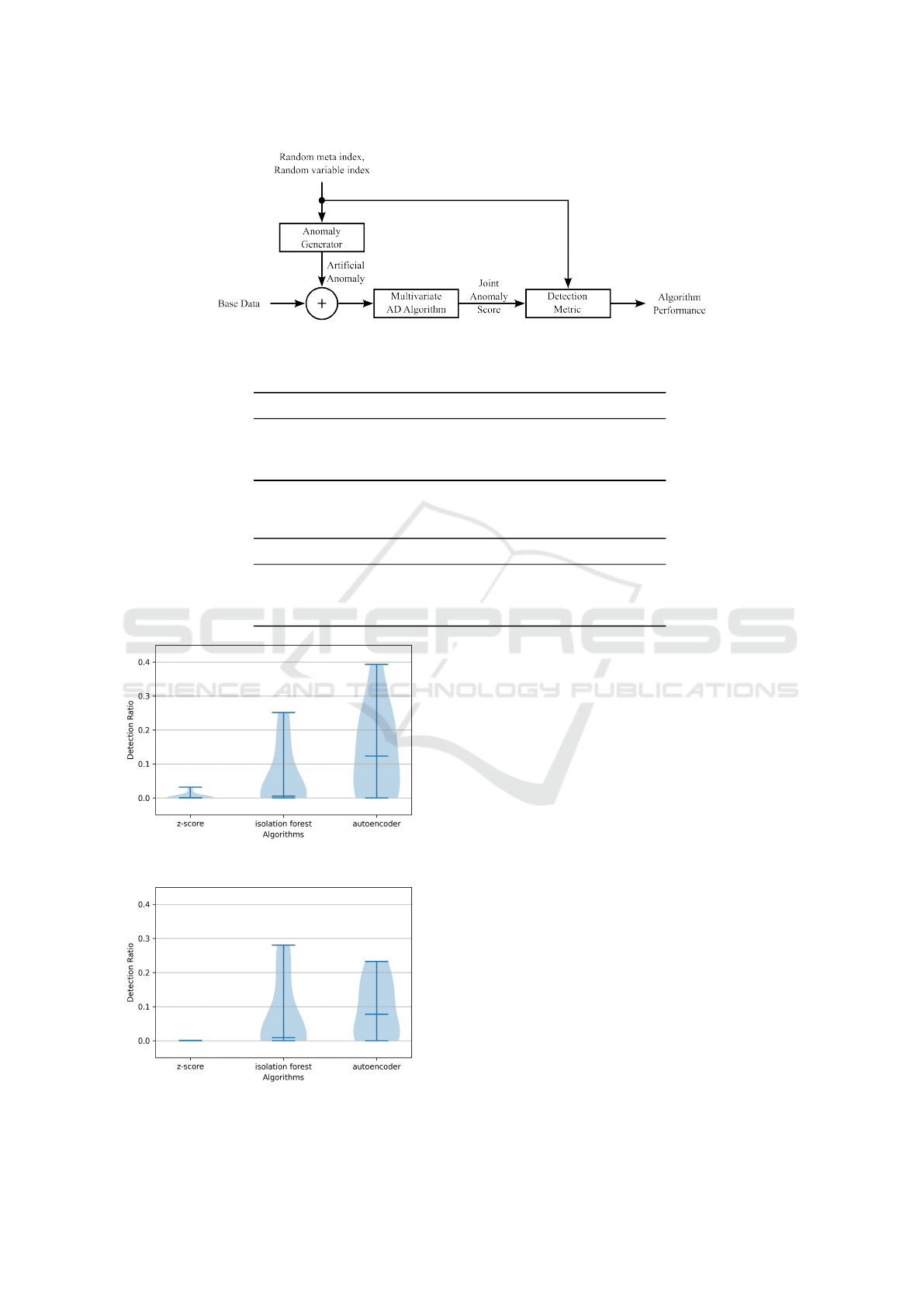
Figure 3: Block diagram of the artificial anomaly experiment.
Table 1: Results table of p-values for the artificial noise data with values rounded to the fifth digit and bold entries for p < 0.05.
z-score isolation forest autoencoder
z-score - 1.0 1.0
isolation forest 7.71964e-56 - 1.0
autoencoder 5.51645e-76 4.61847e-43 -
Table 2: Results table of p-values for the artificial random walk data with values rounded to the fifth digit and bold entries for
p < 0.05.
z-score isolation forest autoencoder
z-score - 1.0 1.0
isolation forest 5.37359e-64 - 1.0
autoencoder 3.80451e-73 4.23226e-08 -
Figure 4: Violin plot of anomaly detection of artificial
anomalies on noise data.
Figure 5: Violin plot of anomaly detection of artificial
anomalies on Gaussian random walk data.
The experiments are organized such that at least
one algorithm is breaking down, due to not detect-
ing the anomalies correctly, on average. Figure 4 and
Figure 5 provide an overview on the results. When
comparing the median values of the detection ratios,
the Autoencoder seems to be the most sensitive of the
three algorithms based on the artificial data experi-
ments. Overall, judging by the Wilcoxon statistics
and the violin plots of the detection ratios, the results
reveal the Autoencoder model to be the best perform-
ing one among the three investigated algorithms, i.e.,
the most sensitive in terms of the outlined experiment.
4.2 Real-World Data Experiment
Three different system platforms were analyzed with
an Autoencoder model and the joint anomaly score S
and individual anomaly scores S
j
were collected dur-
ing the analysis. One specific test case for this inves-
tigation is selected – the so-called startup-time test.
The different performance-data variables consisting
of two system-related ones and twelve container-
related variables. The data is represented according
to the definition in Section 3.2 and referred to as real-
world test case data X
TC
. The startup-time test is
available in a total of I = 1519 CI runs. From its per-
formance data, J = 14 different variables are selected.
Unsupervised Anomaly Detection in Continuous Integration Pipelines
341

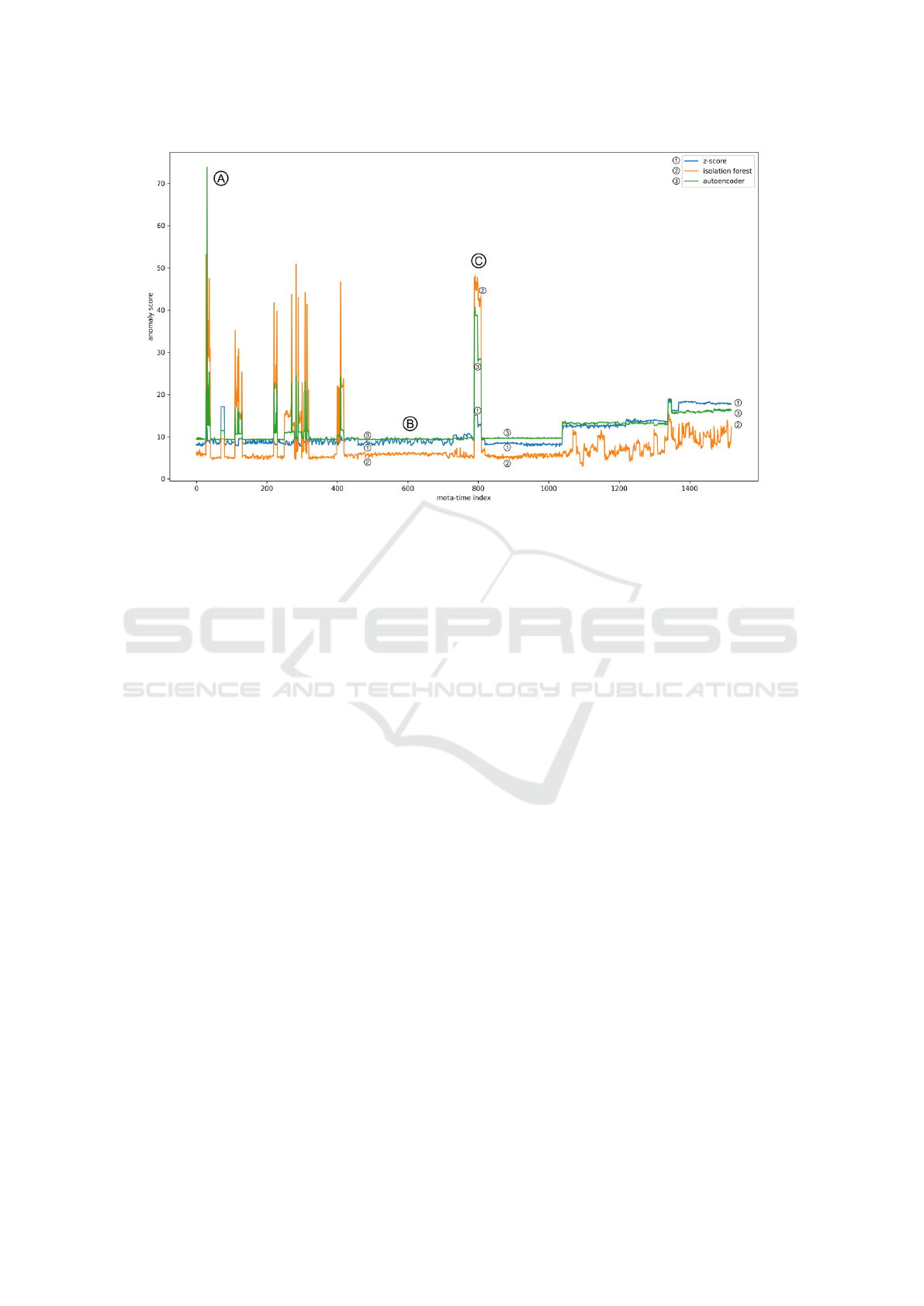
Figure 6: Joint anomaly scores of all CI runs of startup-time tests of one system platform with a distinct peak at meta-
time index 30 (CI run number 31). The algorithms z-score (1), isolation forest (2), and autoencoder (3) are used for their
calculation. The figure also includes three reference points (A, B, C).
The maximum sequence length among all variables is
K = 68.
Due to spacial restriction, the results of only one
of the three analyzed systems is presented in Figure
6. The highest peak of the joint anomaly scores is ob-
servable at meta-time index i = 30. Two of the three
analyzed system platforms show a similar anomaly.
The corresponding test for this anomaly runs signif-
icantly longer than its peers. In fact, the startup-
time test runs 6-times longer than normal, leading to
the detected joint anomaly score (reference point A).
Additionally, judging visually from reference point
B (i = 600), the autoencoder model shows the low-
est variance compared to the other algorithms. This
area is deemed normal by the domain expert. Ref-
erence point C is a point in time (i = 800), which is
labeled by a domain expert (test engineer) as a true
anomaly – occurrence of severe software bugs around
this point in time. As a result, in our opinion, the
Autoencoder strikes a balance between low variance
in normal times (B) compared to distinct scores dur-
ing anomalous times (A, C). Unfortunately only for
the three reference points, the domain expert was able
to track back the results based on his memory. This
weak subjective evidence is obviously not sufficient
for a proper objective analysis, but may at least verify
the overall approach on the given reference points.
5 CONCLUSION
The performance data as part of the CI infrastructure
in the context of embedded software development was
investigated in terms of the identification of poten-
tial software issues. Overall, based on the conducted
experiments, it could be verified on real-world data
that meaningful anomalies for developers and testers
could be identified by means of Machine Learning.
Throughout this work we examined the problem of
identifying anomalies of software performance data
during testing. This is of special interest in the in-
dustry to not only identify failed tests, but also poten-
tial long-term hazards (e.g. memory leaks) that may
not be identified by looking purely at test results (i.e.
passed or failed). Our approach consists out of cre-
ating a schema to multivariate anomaly detection, the
modelling of an appropriate anomaly metric as well
as designing a neural network to identify software is-
sues. From the experiments can be concluded that
the Autoencoder model showed the highest sensitiv-
ity in the artificial experiments, compared to a method
based on z-scores or the isolation forest model. When
applied to the real-word data, the Autoencoder model
is able to detect anomalies confirmed by a domain ex-
pert.
Overall, this paper marks the starting point for fur-
ther investigations. In future work, we ought to ex-
tend this work to a more holistic view of anomaly
ENASE 2024 - 19th International Conference on Evaluation of Novel Approaches to Software Engineering
342

detection, where all tests are considered at the same
time. Either a complementary model can be applied
that deals with inter-variable dependencies or general
algorithms that inherently model these dependencies
can be integrated. In upcoming work, the injection of
memory leaks into the system which is undergoing the
testing procedures would be an interesting study case.
By including more data from real-world projects, bet-
ter thresholds for the decision making may be derived.
This further strengthens the usage of anomaly detec-
tion in CI pipelines.
REFERENCES
Atzberger., D., Cech., T., Scheibel., W., Richter., R., and
D
¨
ollner., J. (2023). Detecting outliers in ci/cd pipeline
logs using latent dirichlet allocation. In Proceedings
of the 18th International Conference on Evaluation of
Novel Approaches to Software Engineering - ENASE,
pages 461–468. INSTICC, SciTePress.
Bourlard, H. and Kamp, Y. (1988). Auto-association by
multilayer perceptrons and singular value decomposi-
tion. Biological cybernetics, 59(4-5):291–294.
BSH Group (2022). Bosch Siemens Home Appliances
(BSH). https://www.bsh-group.com/.
Capizzi, A., Distefano, S., Ara
´
ujo, L. J., Mazzara, M., Ah-
mad, M., and Bobrov, E. (2020). Anomaly detection
in devops toolchain. In Workshop on Software Engi-
neering Aspects of Continuous Development and New
Paradigms of Software Production and Deployment,
pages 37–51. Springer.
Cherkasova, L., Ozonat, K., Mi, N., Symons, J., and Smirni,
E. (2009). Automated anomaly detection and per-
formance modeling of enterprise applications. ACM
TOCS, 27(3):1–32.
Conover, W. (1971). Practical nonparametric statistics.. new
york: Wiley & sons.
Dem
ˇ
sar, J. (2006). Statistical comparisons of classifiers
over multiple data sets. The Journal of Machine learn-
ing research, 7:1–30.
El Amine Sehili, M. and Zhang, Z. (2023). Multivariate
time series anomaly detection: Fancy algorithms and
flawed evaluation methodology. arXiv e-prints.
Fowler, M. (2006). Continuous integration. https:
//martinfowler.com/articles/continuousIntegration.
html.
Garg, A., Zhang, W., Samaran, J., Savitha, R., and Foo, C.-
S. (2021). An evaluation of anomaly detection and
diagnosis in multivariate time series. IEEE Trans-
actions on Neural Networks and Learning Systems,
33(6):2508–2517.
Grigorakis, A. (1997). Application of detection theory to
the measurement of the minimum detectable signal for
a sinusoid in gaussian noise displayed on a lofargram.
Technical report, Citeseer.
Hany Fawzy, A., Wassif, K., and Moussa, H. (2023).
Framework for automatic detection of anomalies in
devops. Journal of King Saud University - Computer
and Information Sciences, 35(3):8–19.
Hrusto, A., Engstr
¨
om, E., and Runeson, P. (2022). Opti-
mization of anomaly detection in a microservice sys-
tem through continuous feedback from development.
In Proceedings of the 10th IEEE/ACM International
Workshop on Software Engineering for Systems-of-
Systems and Software Ecosystems, pages 13–20.
Huck, S. W., Cross, T. L., and Clark, S. B. (1986). Over-
coming misconceptions about z-scores. Teaching
Statistics, 8(2):38–40.
Jorgensen, P. C. (2013). Software testing: a craftsman’s
approach (Fourth Edition). Auerbach Publications.
Jung, C., Lee, S., Raman, E., and Pande, S. (2014). Auto-
mated memory leak detection for production use. In
Proceedings of the 36th International Conference on
Software Engineering, pages 825–836.
Kawaguchi, K. (2011). Jenkins (Software). https://www.
jenkins.io/, accessed on 2023-08-24.
Liu, F. T., Ting, K. M., and Zhou, Z.-H. (2008). Isolation
forest. In 2008 Eighth IEEE International Conference
on Data Mining, pages 413–422.
Provotar, O. I., Linder, Y. M., and Veres, M. M. (2019).
Unsupervised anomaly detection in time series using
lstm-based autoencoders. In 2019 IEEE International
Conference on Advanced Trends in Information The-
ory (ATIT), pages 513–517. IEEE.
Red Hat, Inc. (2022). What is a ci/cd pipeline? https://www.
redhat.com/en/topics/devops/what-cicd-pipeline, ac-
cessed on 2023-12-29.
Sakurada, M. and Yairi, T. (2014). Anomaly detection
using autoencoders with nonlinear dimensionality re-
duction. In Proceedings of the MLSDA 2014, page
4–11. Association for Computing Machinery.
Schmidl, S., Wenig, P., and Papenbrock, T. (2022).
Anomaly detection in time series: a comprehensive
evaluation. Proceedings of the VLDB Endowment,
15(9):1779–1797.
Strandberg, P. E., Afzal, W., and Sundmark, D. (2022).
Software test results exploration and visualization
with continuous integration and nightly testing. In-
ternational Journal on Software Tools for Technology
Transfer, 24(2):261–285.
Tao, X., Peng, Y., Zhao, F., Zhao, P., and Wang, Y.
(2018). A parallel algorithm for network traffic
anomaly detection based on isolation forest. In-
ternational Journal of Distributed Sensor Networks,
14(11):1550147718814471.
Torabi, H., Mirtaheri, S. L., and Greco, S. (2023). Practical
autoencoder based anomaly detection by using vector
reconstruction error. Cybersecurity, 6(1):1.
Wu, R. and Keogh, E. (2021). Current time series anomaly
detection benchmarks are flawed and are creating the
illusion of progress. IEEE Transactions on Knowledge
and Data Engineering.
Yang, Z., Li, H., Yang, X., Peng, H., Shi, J., Peng, M.,
Wang, H., and Bai, H. (2023). User log anomaly de-
tection system based on isolation forest. In 2nd Inter-
national Joint Conference on Information and Com-
munication Engineering (JCICE), pages 79–84.
Unsupervised Anomaly Detection in Continuous Integration Pipelines
343