A Conceptual Model for Data Warehousing

Deepika Prakash

and Naveen Prakash

Institute of Engineering and Technology, Department of Computer Engineering,

JK Lakshmipat University, Jaipur 302026, India

ICLC, 21/3 S, Bhagat Singh Marg, New Delhi 110001, India

Keywords: Analysable Data Type, Type of Analysis Parameter, Historical Analysis Data, Change Type, Conversion,

Star Schema.

Abstract: We show that current approaches for data warehouse conceptual modelling are inadequate for capturing the

range of analysis capabilities of the enterprise. In addressing this, our conceptual model retains the basic

distinction between the analysis data and analysis parameters but additionally introduces intra analysis-data

and intra analysis-parameters relationships besides relationships between analysis data and analysis

parameter. A variety of constraints for enforcing analysis semantics are also defined. We convert the

conceptual model to star schema and show procedures to do so. We illustrate the use of our model through an

example.

1 INTRODUCTION

A data warehouse, DW conceptual schema models

the information contents of the DW to-be and acts as

a specification of its logical data model. There are two

questions (a) what is the set of concepts that comprise

the meta-model and (b) how can a conceptual schema

be converted into the target logical model of data.

One approach has been to adopt (Gol 1998) the Entity

Relationship, ER model. The ER schema is converted

into the Multi-Dimensional, MD, model using the

semi-automatic process presented in (Gol 1998). The

chief difficulty (Boe 1999) with this approach lies in

deciding where to start in the conceptual schema. Due

to this and also since there was no accepted

conceptual model for a DW, (Boe 1999) used the

logical data model comprising facts, dimensions,

dimension hierarchy and integrity constraints, as

their conceptual model. The logical model was

subsequently treated as a conceptual model by several

researchers. In (Cor 2012), dimensions, transactional

facts, periodic and evolving snapshots were

modelled. In (Gio 2008), transactional facts,

dimensions and dimension hierarchies could be

expressed. In (Maz 2007), transactional facts,

dimensions, dimension hierarchies, degenerate facts,

https://orcid.org/0000-0001-8404-3128

https://orcid.org/0000-0003-1644-5613

and degenerate dimensions were adopted.

MultiDimER (Mal 2006) consists of facts,

dimensions, levels, and dimension hierarchies of

various types. A version of this model, MultiDim is

used in (Vai 2022). The conceptual model in (Pra

2018) in addition to facts and dimensions, that they

referred to as data and category objects respectively,

allowed specification of category hierarchies, history

of data objects, and change properties of category

objects.

The major difficulty with using the logical model

is that it is (Kim 1996) specifically structured to

support querying and not towards capturing the

analysis to be carried out. To fill this gap, we

propose a model for capturing the analysis capability

to be supported by the DW. This has two aspects, (i)

semantics of data to be analysed or analysis data, and

(ii) semantics of parameters of analysis. Regarding (i)

we consider five issues as follows:

a. Handling un-structured analysis data. All

conceptual models considered above assume

structured, numeric, additive data, though semi-

additive data is allowed for example in (Cor

2012, Vai 2022). However, analysis of

unstructured data (Fac 2022, Pan 2022) has now

attained importance and must be supported.

Prakash, D. and Prakash, N.

A Conceptual Model for Data Warehousing.

DOI: 10.5220/0012621200003687

Paper published under CC license (CC BY-NC-ND 4.0)

In Proceedings of the 19th International Conference on Evaluation of Novel Approaches to Software Engineering (ENASE 2024), pages 87-98

ISBN: 978-989-758-696-5; ISSN: 2184-4895

b. Specifying relationships among analysis data.

As we will see, these identify the data that must

be analysed together and which must be

analysed separately. These two differing

situations need explicit modelling to capture the

correct analysis.

c. Modelling complex analysis data that shows the

“is-part-of” relationship with its constituent

data.

d. Specifying containment of analysis data, for

example, to model that an Order_Value contains

one or more Order_line_amount.

e. Defining history property of analysis data, i.e,

specifying the duration for which historical data

is to be maintained and its frequency.

There are three issues around (ii) as follows.

f. Specifying specialized analysis parameters

for specific analysis of analysis data. For

example, the parameter, Product may be

specialized into perishable and non-perishable

product respectively thereby allowing separate

analysis of sales data, by perishable and non-

perishable products respectively.

g. Modelling complex analysis parameters to

bring out the “is part of” relationship between

parameters.

h. Modelling containment in parameters to allow

analysis by the container or its contents

respectively. For example, a customer may hold

multiple fixed deposits with a bank. That is, the

customer_id is a container and the several

FD_account_numbers are its contents. Analysis

may be carried out by customer or by individual

fixed deposits.

i. Modelling change properties of parameters

The layout of the paper is as follows. In section 2, we

present the conceptual model including the features

(a) to (i) above. In section 3, we show the conversion

of our model to the star schema. In section 4, we

illustrate its use with a real-life example of a

conceptual schema. Section 5 contains a discussion

and related work. We conclude the paper in section 6.

2 THE CONCEPTUAL MODEL

Our model assumes a separation between analysable

data and parameters of analysis. This separation raises

three questions

• What concepts are needed to capture

analysable data?

• How should parameters of analysis be

modelled?

• What are the relationships between the two?

We consider these in turn.

2.1 Modelling Analysable Data

We propose to introduce the notion of an Analysable

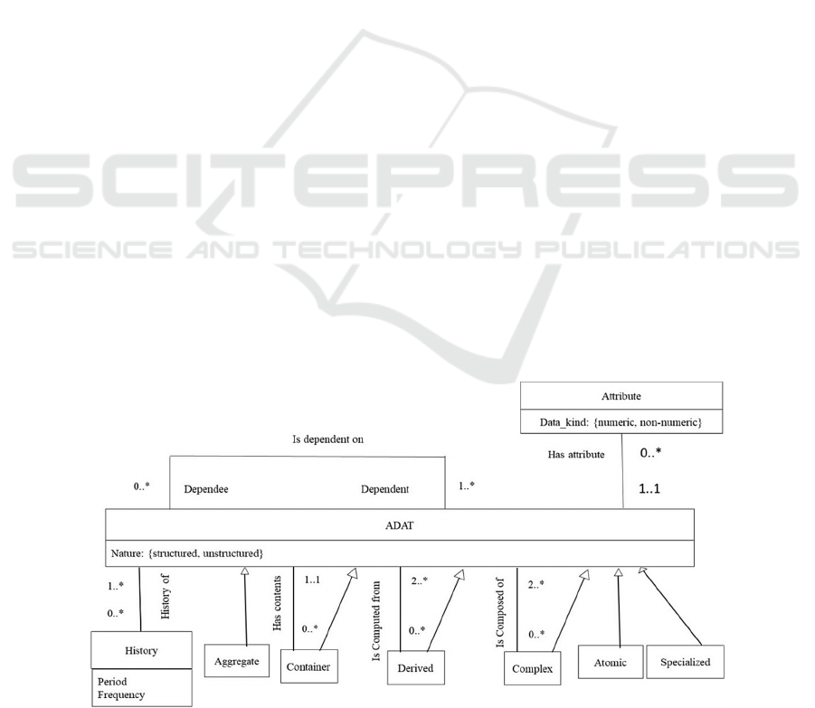
Data Type, ADAT in our conceptual model. The

typology of an ADAT is shown in Fig. 1 in UML

notation. The object type ADAT has a property

Nature that specifies whether the ADAT holds

structured or unstructured data. Further, ADAT has

attributes that contain analysable data. This is

modelled in the figure by the relationship, Has

attribute, between ADAT and Attribute object type.

Attributes are described by Data_kind that defines

whether the data is numeric or non-numeric. With

Nature and Data_kind, it is possible for an ADAT to

hold the following kinds of data:

• Nature = structured and Data_Kind = numeric

(integer, float) or non-numeric (char, varchar);

• Nature = unstructured data and Data_Kind =

non-numeric (such data may be free text, document

etc.);

Notice that the combination Nature = unstructured

and Data_Kind = numeric is NOT PERMISSIBLE.

There are six types of ADATs in Fig. 1, and each

models a specific kind of analysis capability. We

consider each in turn.

1 An atomic ADAT cannot be decomposed into

simpler ones. It has no components and cannot be

decomposed any further. An example of an atomic

ADAT is Sales with attribute, Amount that we

represent as Sales(Amount). Sales is an atomic

ADAT and has no component ADATs. Further, it is

structured and numeric (Amount is a float). As an

example of an unstructured atomic ADAT, consider

Hotel_Feedback(Room_state) that has a non-numeric

attribute, Room_state with a free text value like “the

room was not well ventilated and had a musty smell”.

2 An ADAT may be specialized into its sub types

and participate in an IS-A hierarchy. These sub types

are mutually disjoint. Specialized ADAT inherit

from the generalized ADAT and may have their own

attributes. For example, the ADAT, Sales having

attribute, Amount, may be specialized into Credit

Sales and Cash Sales respectively. Thus, Amount is

inherited by both Credit Sales and Cash Sales. Due to

the specialization being disjoint, Sales is either by

credit or cash and is thus, a way of specifying the

allowed analysis. Specialization can be extended to

unstructured data as well. Consider obtaining

feedback on hotel rooms from two different kinds of

customers, business people and tourists. Feedback

about business centre facilities is obtained from the

former whereas the latter provide feedback on holiday

ENASE 2024 - 19th International Conference on Evaluation of Novel Approaches to Software Engineering

activities. Thus, the generalized ADAT, Feedback is

specialized into two ADATs, Business_facilities and

Holiday_activities, respectively. Again, either one

may be used when analyzing the feedback.

3 A complex ADAT “is composed of” two or

more simpler ADATs and an ADAT may participate

in zero or more than one complex ADAT. The reason

for “two or more” is that defining a complex ADAT

with a single simpler ADAT gives no additional

analysis capability. The simpler ADATs are called

constituent ADATs. Each constituent ADAT has

its own PAN for analysis. An example of a complex

ADAT is Account_statement that consists of ADATs

Credit(Amount) and Debit(Amount). An account

holder can generate, for example, a daily account-

statement showing credit and debits of the day. The

complex ADAT may have its own PANs.

The difference between complex and

generalized ADATs is that when analysing complex

ADATs, we may use, one or more, possibly all

component ADATs, but when analysing a

generalized ADAT, we use only one of its specialized

types.

4 A derived ADAT “is computed from” its base

ADATs. Each base goes into computing the derived

ADAT and must be considered during analysis. An

example with structured, numeric data is the ADAT,

Purchase(Amount).Assume that part payment in

Indian rupees and US dollars is allowed. Amount is

in Indian rupees and is calculated by converting dollar

payment into rupee payment and adding to it the part

payment made in Indian rupees. That it,

Purchase(Amount) is a derived ADAT consisting of

two atomic ADATs, Indian_amount(Ramount) and

US_dollar_amount(Damount). Since part payments

can be made in both currencies, both bases must be

considered during analysis. An example with

unstructured data is the ADAT, Hotel_Feedback with

bases, Room_state and Room_amenities respectively.

The former has the value, “The size of the room is

good. It is carpeted but the carpet needs repair.” The

latter has the value, “Amenities were in good shape.

We asked housekeeping for a hair dryer and it was

delivered to us promptly.” Again, when analyzing,

both bases must be considered to produce the derived

result, for example, “good” if both are good otherwise

“maybe”.

Consider the difference between a derived and

atomic ADAT. If we treat Indian_amount and

US_dollar_amount as attributes of an atomic ADAT,

then (a) it is not specified that both must be used in

deriving the purchase amount and (b) the computed

value is virtual; it is not materialized and is computed

each time it is needed. Derived ADATs are different

from complex ADATs as well. Let us model

Purchase(Amount) as a complex ADAT consisting of

ADATs Indian_rupee and US_dollar_amount. Now,

we can materialize the purchase amount but there is

still no constraint that both must be considered in the

computation. The difference between derived and

generalized ADATs is that when analysing the

former, all base ADATs must be used whereas when

analysing the latter only one of the specialized

ADATs is relevant.

5 A container ADAT is obtained through the

relationship, ‘Has contents’ between ADATs. The

cardinality of the relationship in Fig. 1 shows that

there is only one ADAT object type in a container,

but an ADAT may participate in zero or more

Container ADATs. For example, ADAT Order

contains only one ADAT, Order_line. We impose the

constraint that a container instance must contain one

or more (possibly duplicate) instances of the content

ADAT. Consider an example each of containment in

structured and unstructured analyzable data:

a. The container ADAT, Order is defined for

structured data and keeps a measure of the total value

of the Order whereas the content ADAT, Order_line

keeps the value of the line. Order is a container of

Order_line; there should be at least one instance of

Order_line in an Order. Order value is the sum of the

values in order lines. Order has PANs, Date and

Supplier and in addition, Order_line can be analyzed

by Product_code.

b. For unstructured analysable data, consider the

document, Minutes of Meeting that contains a record

of decisions taken by a committee on various agenda

items as well as the date, place, and list of attendees of

the meeting. The record of decisions is unstructured

text and tells us the decision taken. We express the

foregoing as a container ADAT, Minutes_of_Meeting

with content ADAT, Agenda_record. Each instance of

the former must contain at least one instance of the

latter.

The difference between a container and

complex ADAT is that whereas the former contains

only one ADAT as its contents and a container

instance contains is at least one instance of the content

ADAT, the latter has several ADATs as its

constituents and an instance of the complex ADAT

contains zero or one instance of each constituent

ADAT.

6 An aggregate ADAT is built by performing a

roll-up OLAP operation on an ADAT and a subset of

parameters of analysis associated with it.

As an

example, c

onsider the ADAT Sales analysed by Shop,

Day, Product. We can perform detailed analysis by

determining sales for each day, shop and product.

A Conceptual Model for Data Warehousing

However, we do a roll-up by computing All Sales taken

over the parameter, Product. The result is an aggregate

ADAT, ALL_Product_Sales that tells us the sales of

all products on all days and all shops.

Fig. 1 shows a recursive relationship among

ADATs called, “is dependent on”. This says that

analysis of a dependent ADAT can only be done if its

dependee ADAT exists. As an example, consider

Order and Delivery. Analysis of delivery requires that

there be an order i.e., Delivery is dependent on Order.

One can ask questions like, “which orders have been

delivered beyond their delivery date?” As shown in

Fig. 1, a dependee ADAT has one or more dependent

ADATs and an ADAT may have zero or more

dependee ADATs. The roles, dependee and

dependent are marked in Fig. 1.

Now we can consider how Nature of an ADAT

and Data_Kind of Attribute varies with the different

types of ADATs. Recall that if the Nature of an

ADAT is structured then the data kind of tis attributes

can be numeric or non-numeric. However, if its

Nature is unstructured then the data kind of its

attributes must be unstructured. Consider Derived

ADATs. Since base ADATs are used for computing

a derived ADAT, all base ADATs as well as the

derived ADAT must be of the same Nature. Similarly,

specialized-generalized ADATs have the same

Nature. Again, a container ADAT has the same

Nature as its content. However, a complex ADAT

may have constituents that are of varying Nature.

If any constituent is unstructured then the

complex ADAT is unstructured else if any constituent

is structured, non-numeric then complex ADAT is

structured, non-numeric else it is structured numeric.

Fig. 1 shows that the type, History has two

attributes, period and frequency. This allows the

modeler to specify the number of years and frequency

of history of an ADAT needed for analysis. The

“History of” relationship allows history to be

optionally maintained for an ADAT as shown by the

0..* cardinality but, in the reverse direction, History

must be associated with at least one ADAT. As an

example of the use of history, let there be an ADAT,

Purchase. We may want to keep a history of monthly

purchases for a period of five years as well as quarterly

history for five years. Thus, we have the ADAT,

Purchase in a “history of” relationship with H

and H

;

has the attribute Period=5 years and Frequency =

Month whereas H2 has Period = 5 years and Frequency

= Quarter. In the reverse direction, an instance of

History may be associated with one or more ADATs.

Thus, we may want to keep history of both monthly

purchases and monthly sales for 5 years. Clearly, H

has two ADATs associated with it.

2.2 Modelling Analysis Parameters

A PAN, Parameter of ANalysis, of Fig. 2 refers to a

type of parameter. The object type PAN has attributes

as seen by the “is property of” relationship between

PAN and PAN_Attribute types. The cardinality

shows that each PAN should have at least one

PAN_Attribute type that is described by Change

Type. This identifies the action to be taken when the

value of the attribute changes. Change Type takes on

values from {update, no_update}. The first value,

update, says that a change in the value of the

PAN_attribute is treated as an update and the original

value is over-written. The second value, no-update,

says that update is not allowed. Instead, the change is

treated as the creation of a new instance of PAN such

that its PAN_attribute has the new value. The

previous PAN instance is not deleted.

Figure 1: Analyzable Data Type, ADAT.

ENASE 2024 - 19th International Conference on Evaluation of Novel Approaches to Software Engineering

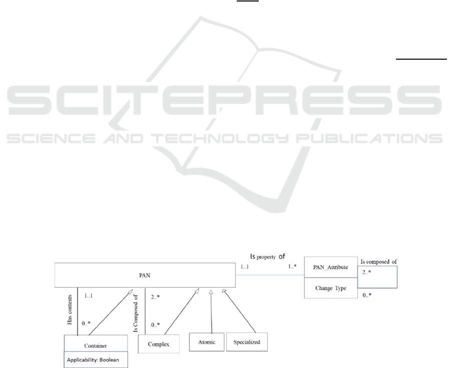
Now, Fig. 2 shows that there are the following

four types of PANs:

1. An atomic PAN cannot be decomposed into

simpler ones. For example, Product is an atomic PAN

having Attribute, colour whose Change Type =

update.

2. A complex PAN shows a “is composed of”

relationship between PANs. Fig. 2 shows that a PAN

may participate in zero or more complex PANs and

that a complex PAN is built over two or more simpler

PANs. For example, the complex PAN, Product is

built over simpler PANs, Product_specification and

Product_description.

3. Fig. 2 shows that a container PAN is built over

exactly one content type of PAN. We impose the

constraint that an instance of the container PAN

must have one or more distinct instances of its

content PAN; distinct because replication does not

enhance analysis. A container PAN is like a container

ADAT except that it contains only distinct instances

of its content PAN whereas duplicate instances are

allowed for ADATs. Consider a group of companies

that consists of subsidiary companies. There are two

ways in which any purchase can be analysed, by

individual subsidiaries or by the group. If a

subsidiary makes a purchase then the purchase is

analysed by the subsidiary but possibly also by the

group company. Similarly, the group may make

purchases for allocation to its subsidiaries. Again,

analysis may be made by the group company and

perhaps, by the subsidiary. The specification of

whether analysis is by the group company or

subsidiary or both is considered in section 2.3.

4. A specialized PAN inherits from the generalized

PAN and has its own attributes. Specialization splits

the generalized PAN into disjoint partitions. This

allows analysis by any of the specialized PANs. For

example, the PAN, Product is specialized into disjoint

partitions, Perishable Product and Non-perishable

Product.

2.3 The “Is-Analysed-by Relationship

The “is analyzed by” relationship of Fig. 3 associates

attributes of ADATs with PANs. In effect, this

relationship says that ADATs can be analysed by

PANs. The cardinality of this relationship shows that

(a) an ADAT may be analyzed by one or more PANs

and (b) a PAN may have one or more ADATs which

it analyzes. Whereas, the relationship makes it

possible to identify the PANs of an atomic ADAT,

this determination requires careful consideration for

the other five kinds of ADAT. This is because of

“interfering” PANs that arise due to the structures of

these ADATs. Determination of PANs for ADATs is

done by rules as follows:

• An atomic ADAT has its own PANs as

parameters.

• The derived ADAT and its bases have the

same PANs. For example, the derived ADAT,

Purchase as well as its bases, Indian_rupee_purchase

and US-dollar_purchase have the same PANs,

namely, Product, and Vendor.

• A complex ADAT and its constituent ADATs

may have PANs that are common but, additionally,

both may have their own specific PANs.

• Generalized ADATs have their own PANs.

Specialized ADATs inherit the PANs of their

generalized ADAT and, additionally, have their own

PANs. Consider Sales_amount specialized into

Cash_sales and Credit_sales. Let Sales_amount have

PANs, Product, Customer, and Date. These are

inherited by both, Cash_sales and Credit_sales.

Additionally, Cash_sales has its own PAN, Currency

and Denomination in which sales were made whereas

Credit_sales has the PANs, Credit_card type,

Cardholder’s_name. Thus, applying our rule,

Cash_sales has parameters Product, Customer,

Date, Currency, and

Denomination whereas

Figure 2: Parameter of Analysis, PAN.

A Conceptual Model for Data Warehousing

Credit_sales has Product, Customer, Date,

Credit_card_type, and Cardholder’s_name.

• Container and content ADATs have their own

PANs. Consider the Container ADAT, Order and

its Content, Order_line. Order is associated with

PANs, Supplier, Order_date, Delivery_terms.

Order_line has PAN, Product.

• An aggregate ADAT has PANs that are a subset

of the PANs of the ADAT from which they have

been aggregated. The PANs that did not participate

in the aggregation are the PANs of the aggregate.

The attributes of “Is analyzed by” makes precise the

semantics of analysis. As shown in Fig 3, there are

three analysis properties, Additivity, Cardinality and

Applicability. Applicability specifies whether

constituents of a complex PAN or content PANs of a

container PAN can be used to analyse the ADAT

associated with the complex or container PAN

respectively. Applicability is specified in the

complex/container PAN, and it is possible for analysis

to be done by constituent/content PAN when

Figure 3: Relating ADATs and PAN.

Applicability=True. Consider the container PAN,

Group of Companies and its content, Subsidiary

Companies. Let material be purchased for the entire

group. Therefore, analysis of purchases is for Group

Companies. However, subsidiary companies are

permitted to analyse the purchases made as well. Thus

Applicability = True. Now, consider that the group,

GC makes purchases for the group. All analysis is

done by Group Companies and purchases are not

analysable by Subsidiary Companies. Now,

Applicability=False.

The attribute, Additivity is Boolean valued.

Consequently, it is possible to specify that an attribute

of an ADAT is additive/non-additive along a PAN or

not. Evidently, when an attribute is non-numeric then

analysis is non-additive along all PANs and, by

default, Additivity = False for all. On the other hand,

when it is numeric then additivity must be specified.

For example, consider the attribute,

Available_balance of ADAT, Account. Let Account

have two PANs, Customer and Month as its

parameters. We can compute the total

Available_balance in all accounts of a Customer.

Thus, Additivity=True for the Available_balance –

Customer relationship. However, when analysis is

done on Month then Additivity=False because we

cannot sum the previous end-of-month balances to

obtain the available balance in the current month.

The remaining analysis property of Fig. 3 is

Cardinality. It is used for specifying the cardinality

of an instance of the “is analyzed by” relationship.

We adopt the conventions of UML notation here.

Consider that Sales_amount of ADAT Sales is

analyzed by Salesperson. It is possible that a sale is

done directly, without involvement of any

salesperson, it is done by a single salesperson, or it is

done jointly by several salespersons. In the reverse

direction it is possible that a salesperson does zero or

more sales. Thus, the cardinality of the relationship is

0..* : 0..*.

Analysis by container and content PANs is

constrained by two rules,

a. An attribute of an ADAT analysable by a content

PAN can be rolled up using the container PAN and

then drilled down to the content PAN. For example,

let there be an attribute, Amount of ADAT, Sales, Let

its PAN be Day. The container PAN, Week contains

Day. We can roll-up Amount to get Monthly_sales.

Vice versa, the latter can be drilled down to get

Amount of sales on a day.

b. An attribute of an ADAT can be associated with a

container/complex PAN. Analysis by these is

allowed if Applicability=True.

2.4 Is Obtained from

This relationship, see Fig. 3, says that a PAN can be

obtained from zero or one ADAT whereas an ADAT

may contribute to zero or more PANs. As an example,

consider determining the discounts price offered to

customers whose annual purchase is more than

100,000 Indian rupees. Sale amount and discount

information is available in the ADAT, Sales. We

define an atomic PAN, Annual_sales and obtain its

value by deriving it from Sales, (a) create an

aggregate ADAT, Yearly_sales and (b) introduce it as

the attribute of Annual_sales. Similarly, one can use

Containers, e.g., to analyze the behaviour of

customers holding combined balance in all accounts

above a certain threshold. Again,

Total_customer_balance is obtained from the ADAT

and introduced in a PAN.

NOTATION: The notation used for representing

the schema is UML based, i.e., UML object notation

ENASE 2024 - 19th International Conference on Evaluation of Novel Approaches to Software Engineering

for ADATs, PANs as well as their attributes; UML

aggregate notation for complex ADAT/PAN; (c)

UML arrow for specialized ADAT/PAN. However,

for derived ADAT, we introduce UML arrow head

containing the letter D at the derived ADAT end, and

arrow head containing the letter C at the container end

for containment of ADAT/PAN. This notation is used

in the example schema of Fig. 4 in section 4.

3 GETTING THE STAR SCHEMA

The logical data model of a data warehouse can either

be a star or snowflake schema. However, the star

schema is the preferred one except in certain specific

situations (Ada 2010, Kim 1999). Therefore, we

present our approach for converting our conceptual

schema to the star schema. Our tool takes an

expression of the conceptual schema as a CSV file

and produces the DDL script for the star schema in

the relational model.

In this section, we show the procedures for

handling the different types of PANs and ADATs and

inter-relationships between then during conversion.

3.1 Converting Atomic PANs to

Relations

Consider an Atomic PAN. The procedure is given in

Table 3.1, which inputs one Atomic PAN, P and

outputs one relation, R. Step 1 of the procedure thus,

creates a relation R for atomic PAN P. Now, from the

PAN meta-model, each PAN can have 1..* Attributes.

When moving to the relational model, every Attribute

of P is added as a column to R (step 1.a.i). The domain

of the column can be appropriately chosen. Next is

Change Type for each Attribute which is either

{update, no_update}. In the case of the latter, we add

another column, Ai_Timestamp, a timestamp

column, to mark the time of update of Ai(step 1.a.ii).

In the case of the former, no schema change has to be

made since an update on the data is desired.

The ‘is composed of’ between attributes, attribute

Ai is composed of Aj, is mapped in step 1.b by the

function PANAttribute_Attribute. A new relation,

PANAttribute, is created to store this hierarchy and

each ‘is composed of’ instance is stored as a tuple in

this relation.

Lastly, for every relation R, we add one surrogate

key (step 1.d).

Table 3.1: Procedure to convert Atomic PAN.

Input: Atomic PAN, P

Output: Relation,

step 1: create a relation R for P

a. for ever

Attribute, Ai, of P

i. addColumn (Ai)

ii. if (chan

pe == no

update)

addColumn (Ai

Timestamp)

end i

end for

b. create a relation PANAttribute_Attribute

c. fn: PANAttribute_Attribute (Ai)

for ever

Ai “is composed of” A

i. insert_tuple_PANAttribute_Attribute(Ai,

Aj)

ii. if Aj ‘is composed of’ Ak

PANAttribute

Attribute(A

)

end for

d. createAddSurro

ateKe

(R) as Primar

3.2 Converting Specialized PANs to

Relations

A specialization gives rise to a tree and it is therefore

important to examine which node of the tree is in a

“is analyzed by” relationship with the ADAT. Based

on this, three cases arise:

Case 1. The root node of the PAN specialization

tree is connected to the ADAT.

Case 2. Any intermediate PAN node is in a

relationship with the ADAT.

Case 3. ALL the PAN nodes in the tree are in their

own separate relationship “is analyzed by” with the

ADAT.

We will consider each in turn.

Case 1: Not only the root PAN, but all PANs in the

hierarchy are analysis parameters for the ADAT “Is

analysed by” the root. This implies that there is a

single relation in which each node is represented, or,

in other words, the tree is flattened. Table 3.2 (a)

shows the procedure for the conversion.

The root PAN is converted to a relation, R (step

1). For every child, ci of a parent PAN, the attributes

are added as columns of R (step 2.b.i.1). Change type

of every attribute is processed as before (step 2.b.i.2).

Also, if a child PAN does not have any specialized

attribute, then a Boolean attribute is added to record

the presence of the PAN in the tree (step 2.a). Finally

for every child PAN, a surrogate key is created and

added to R (step 2.c).

Notice, a denormalized table is created. Notice

also that in the PAN model, it may often be the case

that only one subtree may have nodes. Therefore,

A Conceptual Model for Data Warehousing

when translated, we may end up with NULLs in our

relation R. Another design choice would be to keep

the specialization tree as it is and create a separate

relation for each PAN giving us R1,R2,,,Rn. In other

words, create a denormalized schema but we reject

this because it leads to a snowflake and not a star

schema.

Table 3.2 (a): Procedure to convert Specialized PAN.

Input: Specialized PAN tree, T

Output: Case1 & 2: Single Relation; Case3: Set

of Relations

Case 1

fn: createSpecializedLevelCase1 (node)

step 1: if (node == root)

follow step 1 of Atomic PAN and create a relation,

R, for root PAN

step 2: for ever

child PAN, ci, of node

a. if (ci does not have an

specialized attributes)

alter R to add a Boolean column for ci

. else

i. for ever

attribute, ai, of ci

1. alter R to add text column, ai, for ci

2. if (chan

pe == no

update)

addColumn (Ai

Timestamp)

end if

c. alter R to add surro

ate ke

of ci

d. if (the sub tree of ci is not empt

)

createSpecializedLevelCase1 (ci)

end for

Case 2: Since an intermediate PAN node analyses the

ADAT, all PANs in the sub-tree rooted in it as well

its parent, grandparent etc. till the root of the tree, are

analysis parameters as well. The pseudocode for

conversion to star schema is shown in Table 3.2(b).

The intermediate PAN, input, is converted to a

relation, R (step 1). Again, for this, step 1 of the

procedure of Atomic PAN is used. The attributes of

the parent node are added to R (step 2). Change type

for each attribute is captured (step 2.a.ii). A surrogate

key is created for each node in the parent hierarchy

and added to R (step 2.b). The process of adding the

subtree attributes to R is the same as Case1. Notice,

as before, change_type for each attribute as well as

the surrogate key for each child is added to R as well

(step 3.c).

Case 3: Here every PAN analyses an ADAT

separately, it can be treated as an atomic one, entering

into its own ‘is-analysed-by’ relationship. Therefore,

we create a new relation for every PAN in the tree

following the procedure of Table 3.1. PAN attributes

are the UNION of inherited as well as its own

attributes. After conversion, we get as many star-

schemas as the number of nodes in the specialization

tree.

Table 3.2(b): Specialized PAN conversion Case 2.

Case 2: ADAT - is analysed by intermediate PANs

fn: createSpecializedLevelCase2 (input)

step 1: follow step 1 of Atomic PAN and create a

relation R for input PAN

ste

2: for ever

arent PAN,

i, of in

ut PAN

a. for every attribute, ai, of pi

i. alter R to add ai as a text column for ci

ii. if (change_type == no_update) then

addColumn

(

Timestam

, R

)

end if

end for

b. alter R to add surrogate key of pi

c. createForChild

(

)

fn: createForChild (input)

ste

3: for ever

child PAN, ci, of in

ut PAN

a. if (ci does not have any specialized attributes)

alter R to add a Boolean column for ci

. else

i. for every attribute, ai, of ci

alter R to add text column, ai, for ci

if (change_type == no_update) then

addColumn (ai_Timestamp. R)

c. alter R to add surro

ate ke

of ci

d. if (the sub tree of ci is not empty)

createForChild (ci)

end for

3.3 Converting Other Kinds of

Multi-Level PANs

Container and complex PANs also result in PAN

hierarchies. Consider container PANs. The surrogate

key is created for the container/content PAN

connected to an ADAT via the “is analysed by”

relationship. The procedure of Table 3.2(b) needs

only to be altered. The procedure is called with the

container/content PAN connected to an ADAT. Steps

1 and 2 remain the same for creating the relation R.

The word ‘parent’, in step 2, is changed to

‘container’. However, we modify the createForChild

function to accommodate setApplicability property,

see Table 3.3.

Now, consider a complex PAN. We create a

relation, R, for the complex PAN using the procedure

in Table 3.1. Its constituent PAN/s is/are included in

R as attributes.

PAN hierarchies can be a mix of various types of

PANs as well. For a structure with a mixed set of

PANs, we follow the procedures as given in the

Tables 3.1

to 3.3. If a relation with the same name

ENASE 2024 - 19th International Conference on Evaluation of Novel Approaches to Software Engineering

Table 3.3: Modified createForChild.

fn: createForChild (input)

step 3: for ever

conten

PAN, ci, of input

a. for ever

attribute, ai, of ci

alter R to add text column, ai, for ci

if (change_type == no_update) then

addColumn (ai

Timestamp. R)

. setApplicability(value)

c. alter R to add surro

ate ke

of ci

d. if (the sub tree of ci is not empt

)

createForChild (ci)

end for

already exists then, (a) merge the relations, (b) the

columns of the merged relation are the union of the

merged relations.

3.4 Converting Atomic ADAT to

Relations

Having finished with PANs, we consider procedures

for converting atomic ADATs into relations. The

procedure shown in Table 3.4 takes an ADAT D as

input, creates a relation R for it and includes attributes

of D as attributes of R. The function detDataType

takes Data Kind and Nature as arguments and gives

data types of relational attributes (step 1.a). The

function, addAdatKey() creates a unique key for R

(step 1.b). This is equivalent to the FACT key. The

surrogate key for every PAN in an ‘is-Analyzed-by’

to the ADAT, D is added in R as a column (step 1.c.i).

The Additivity property is recorded using the function

determineAdditive (step 1.c.ii). If the cardinality is

zero, then a special surrogate key is created (step

1.c.iii). This key is inserted into R with other columns

having NULLs or default values. Lastly, the ‘is-

obtained-by’ relationship is converted as shown in

step 1.d. Completion of the Entire Procedure Gives

us a Complete Star Schema.

3.5 Converting Specialized ADATs to

Relations

Since ADATs may be analysed by different PANs in

a tree, we create a relation for each ADAT node using

the procedure in Table 3.5. The attributes of the child

node are the UNION of the inherited attributes as well

as its own specialized attributes. Notice, we get as

many star scheme as the number of nodes in the tree.

However, in order not to lose the semantics of the tree

structure, we modify the procedure of Table 3.5 to

add step 2, as given below:

Step2: create table if not exists specializedADAT

(ParentADAT text, childADAT text)

Step 2.1: insert tuple into specializedADAT

Table 3.4: Procedure to convert Atomic ADAT.

Input: Atomic ADAT, D

Output: Single Relation R

step 1: create a relation R

a. for ever

Attribute, Ai

addColumn(Ai,detDataT

pe(DataKind,Nature)

end for

. addAdatKe

() as primar

c. for ever

is-

nal

zed-b

relationship

i. addColumnSurro

ateKe

(PAN

SK)

ii. determineAdditive (ADAT,

ADAT

Attribute, PAN, additive)

iii. if (cardinalit

.Contains(0))

createAndInsert

newPANSurro

ateKe

= Default value into the PAN

end for

d. for ever

is-Obtained-b

relationship

addColumnAdatKe

()

end for

fn: determineAdditive (ADAT, ADAT_Attribute,

PAN, additive)

step i: create a relation if not exists is_Additive

with columns ADAT_name, ADAT_Attribute,

PAN, is

Additive)

step ii: if (Data

Kind = = non-numeric) then

insert into is_Additive the values with

Additive = “false”

else

insert into is_Additive the values with

Additive = “true”

3.6 Converting Other Multi-Level

ADATs

For a containment, the container and content have

their own separate PANs or may have exactly the

same PANs. In either case, we create separate

relations for every ADAT. To capture the relationship

between container and content, for the former case, a

separate relation is created while for the latter case,

the container surrogate key is added to the content

PAN.

Let us consider the case of Derived ADATs. All the

PANs associated are the same through-out the

hierarchy. We create separate relations, one for the

root derived ADAT, and one for each “Derived”

symbol, which is point of merge of several base

ADATs. The latter is done because the base nodes

are used in the calculation of the derived node. The

procedure is shown in Table 3.5.

A Conceptual Model for Data Warehousing

Table 3.5: Procedure to convert Derived ADAT.

Input: Derived multi-level ADAT

Output: Set of Relations

step 1: follow step 1 of Atomic ADAT and

create a relation R for roo

ADAT

step 2: for ever

mbol D

a. create a relation name derived-

ase i-(n)

. for ever

base ADAT, bi

for ever

attribute, ai, of

add column to derived-

ase i-(n)

end for

addAdatKey() as composite primar

c. alter R: add composite AdatKey as foreign

key

end for

For complex ADAT, the complex and the constituent

have at-least the same PANs and in addition may have

other PANs. Therefore,

• if no additional PANs are associated, then the

same procedure as Table 3.5 is used. The only

change is in step 2 where the symbol changes to

the complex symbol of the letter c contained in a

triangle.

• if additional PANs are associated at any level,

then separate relations are created and the

semantics of the relationship is captured in a

separate relation as in the case of specialization.

Finally in the case of a mixed structure, we apply a

priority to every type of ADAT, which is:

1. Containment, Specialization, Derivation type are

at the same priority.

2. Complex type is given a higher priority.

The lowest priority is zero. We start at the bottom and

scan the mixed structure for Containment,

Specialization, Derivation type of ADATs and assign

them a priority of 0. The first set of Complex type

from the bottom is given priority of 1. The next set of

Containment, Specialization, Derivation type of

ADATs, going up in the hierarchy, is assigned a

priority of 2. The complex type thereafter gets a

priority of 3. This continues till the root of the mixed

structure.

After assigning priorities, we convert the specific

ADAT types into relations using their specific

procedures. We start the iteration with priority of

zero. ADAT types at the same priority can be picked

at random for conversion based on domain

knowledge. If any two relations with the same name

exists, then we rename one of them. We avoid

merging as the associated PANs may be different.

4 EXAMPLE

A film company releases movies internationally,

across different countries. It produces, distributes, and

markets its films. The company is also interested in

the revenue generated from cinema-goers on sale of

tickets. The contract may also be signed with a chain

of cinema halls for screening the film in all its halls.

If cinema halls are independent, then the contract is

signed with these independent entities. A data

warehouse for analysing these is to be conceptualized.

The full schema consists of four parts, Production,

Distribution, Marketing, and Revenue. For reasons of

space, we show Production and Distribution only, see

Fig. 4. We represent expenditure of crew member as

the ADAT, crewCost. crewCost is a derived ADAT of

two ADATs, namely, transportCost and

professionalFees; crewCost “is analyzed by” atomic

PANs movie, and date. The PAN, crew is specialized

into atomic PANs, actor, director, technicalStaff. In

Fig. 4, additivity and cardinality are not shown to

avoid graphical clutter.The cardinality for movie :

crewCost :: 1..1 : 1..*; for date: crewCost:: 1..1 : 0..*;

for crew:crewCost :: 1..1: 1..*.

Fig. 4 also shows the schema for distribution. Contract

is represented as a complex ADAT with three

component ADATs, paymentTerms,

paymentSchedule, and termsAndConditions. ADAT

paymentTerms is a container of the atomic ADAT,

paymentTermLine. Similarly, paymentSchedule is a

container of the atomic ADAT,

paymentScheduleLine. ADAT termsAndConditions is

a container of terms and condition clauses, i.e., of the

atomic ADAT, TandCClauses. As shown, these are

unstructured. Contract is analyzed by the atomic

PANs movie, and cinemaHall. PAN cinemaHall is

contained in the container PAN, cinemaChain. For

uniformity, we have assumed hotel chains, each with

a single cinema hall for individual cinema halls also.

cinemaChain has Applicability=True and contracts

can be analyzed by cinemaHall. For both movie-

contract and cinemaHall-contract, Additivity = False

and cardinality for movie:contract::1..1:1..*; for

cinemaHall: contract:: 1..1 : 1..1. As before, these are

not shown in the figure.

We show the conversion of

crewCost in Fig. 5. Procedures discussed in section 3

were applied. Movie and Date are Atomic PANs.

Since there was no ‘is-composed-of’ between PAN

attributes, no tuple is inserted into the

PANAttribute_Attribute relation. Crew is a

specialized Case I type of PAN and therefore, all the

attributes of director, actor and technicalStaff are

added to the relation crew.

ENASE 2024 - 19th International Conference on Evaluation of Novel Approaches to Software Engineering

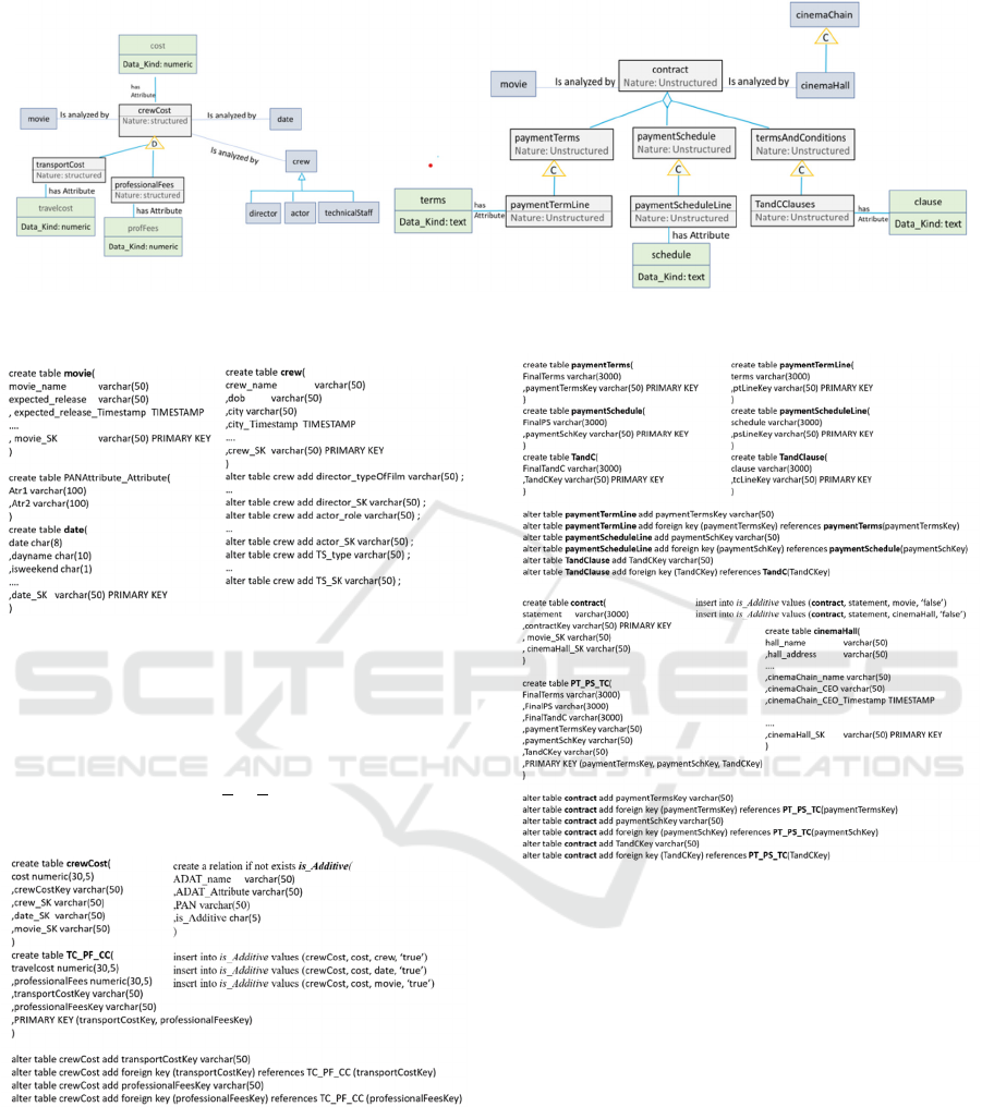
Figure 4: Instantiation of the model showing crewCost and Contract.

Figure 5: (a) DDL script for PANs movie, date and crew.

crewCost is the root derived ADAT and so a relation

is created with ‘cost’ and surrogate keys of movie,

date and crew. For Additivity, a tuple is inserted for

each ‘cost’-PAN-true/false pair in the relation is-

Additive. A relation TC PF CC is created for the

“Derived Symbol”, with the attributes of transport

cost, professional fees and a composite key.

Figure 5: (b) DDL script for crewCost schema.

Contract is a ‘mixed’ multi-level ADAT structure.

The three container ADATs get a priority of 0 and

Contract a priority of 1. Out of 0s, paymentTerms is

selected first and the container/content procedure is

applied. Notice, that there is no specific ‘is-analyzed-

by’ associated with this ADAT and so no PAN

surrogate keys are added to the relation. At the next

level, Contract is converted as shown in Fig 6.

Figure 6: DDL script for Contract schema.

5 DISCUSSON

Whereas traditional conceptual modelling is used to

represent system functionality of information and

software systems, its use in DW is to represent the

analysis capability to be supported. There are two

distinct concepts, ADATs and PANs for the latter,

whereas in information/software systems there is only

one concept, object type. In both types of conceptual

modelling, we have some common features like

association, dependency, and specialisation but in the

DW context their interpretation is done to specify

how data can be analysed. It is not merely for

capturing data and its inter-relationships as in

information/software.

A Conceptual Model for Data Warehousing

Much attention was given in DW on BI tool

operability and meta-models. like the Common

Warehouse Model, CWM (OMG 2003), that abstract

out common features of logical models of BI tools

were developed. These meta-models only considered

structured data. Several proposals that use object

modelling concepts for their meta-models (Li 2005,

Tru 2000) were also made. The basic idea was to

represent facts and dimension as object classes. In

(Tru 2000), the fact/dimension relationship is treated

as a UML aggregation. Li and An (Li 2005) do XML

Schema conversion into UML and propose an

integration tool for formulating OLAP queries.

While allowing tool interoperability the attempt, in

the foregoing, was not to model the required analysis

capability. Consequently, the use of concepts like is-

part-of, containment, and ISA relationships for

analysis are not available there. While CWM allowed

time stamping of data, specifying periodicity and

duration is not possible. However, change properties

can be specified in CWM.

In (Ban 2021), we have an abstract model for

NoSQL databases to facilitate representing data

warehouse logical model in such data stores. Again,

this is a common meta-model for converting to

specific NoSQL data stores and the model does not

express analysis needs.

In recent years we have seen emergence of multi

model data warehouses (Bim 2022). Since we

conceptualize different kinds of data, our model

provides an abstraction using which multi model data

warehouses can be built.

6 CONCLUSIONS

We have developed a conceptual model for analysis

tasks for analysing structured and unstructured

ADATs. Inter-ADAT relationships specify related

analysis data; inter-PAN relationships specify the

structure of analysis parameters, and ADAT-PAN

relationships model what can be analysed by what

parameter. We have presented rules for conversion to

the star schema. In future, we shall develop rules for

converting to column-oriented relational databases.

REFERENCES

Adamson C., Star Schema: The Complete Reference, Tata

McGraw Hill, 2010

Banerjee S., Bhaskar S., Sarkar A., Debnath N.C., A

Unified Conceptual Model for Data Warehouses,

Annals of Emerging Technologies in Computing,162-

169, 2021

Bimonte S, Gallinucci E., Marcel P, Rizzi S., Logical

design of Multi-Model Data Warehouses, Knowledge

and Informaiton Systems, Knowledge and Information

Systems https://doi.org/10.1007/s10115-022-01788-0,

2022

Boehnlein, M., and Ulbrich vom Ende, A. Deriving initial

Data Warehouse Structures from the Conceptual Data

Models of the Underlying Operational Information

Systems, in Proc. Of Workshop on Data Warehousing

and OLAP, 15-21, 1999

Corr L., Stagnitto J., Agile Data Warehouse Design,

Decision One Press, UK, 2012

Faccia, A., Cavaliere L.P.L., Petratos P., Mosteanu N.R.,

Unstructured Over Structured, Big Data Analytics and

Applications In Accounting and Management.

In Proceedings of the 2022 6th International Conference

on Cloud and Big Data Computing, 37-41. 2022.

Giorgini P., Rizzi S., Garzetti M., GRAnD: A goal-

oriented approach to requirement analysis in data

warehouses. Decision Support Systems, 45(1), 4-21,

2008

Golfarelli, M., Rizzi, S.: A methodological Framework for

Data Warehouse Design. In: Proc. of the ACM 1st Intl.

Workshop on Data warehousing and OLAP

(DOLAP’98), Washington D.C., USA, 3–9, 1998

Kimball R., The Data Warehouse Toolkit, Wiley, 1996

Li, Y., An, A., Representing UML Snowflake Diagram

from Integrating XML Data Using XML Schema,

Proceedings of the 2005 International Workshop on

Data Engineering Issues in E-Commerce, 103 – 111,

2005.

Malinowski E., Zima´nyi E., Hierarchies in a

multidimensional model: from conceptual modeling to

logical representation, Data & Knowledge Engineering

59 (2) 348–377, 2006

Mazón, J. N., Pardillo, J., & Trujillo, J. A model-driven

goal-oriented requirement engineering approach for

data warehouses, in Advances in Conceptual

Modeling–Foundations and Applications, 255-264,

Springer, 2007

Object Management Group, Common Warehouse

Metamodel Specification, Version 1.1, Vol 1, 2003

Pantano, E., Dennis, C., & Alamanos, E., Retail managers’

preparedness to capture customers’ emotions: A new

synergistic framework to exploit unstructured data with

new analytics. British Journal of Management, 33(3),

1179-1199. 2022

Prakash D., Direct Conversion of Early Information to

Multi-dimensional Model, DEXA, 19-126, 2018

Trujill J., Palomar M., Gómez J., Applying Object-

Oriented Conceptual Modeling Techniques to the

Design of Multidimensional Databases and OLAP

Applications, Web-Age Information Management, 83-

94, 2000

Vaisman, A., Zimányi, E., Conceptual Data Warehouse

Design. In: Data Warehouse Systems. Data-Centric

Systems and Applications. Springer, https://doi.

org/10.1007/978-3-662-65167-4_4, 2022.

ENASE 2024 - 19th International Conference on Evaluation of Novel Approaches to Software Engineering