An Evaluation of Pre-Trained Models for Feature Extraction in Image

Classiﬁcation

Erick da Silva Puls, Matheus V. Todescato

and Joel L. Carbonera

Institute of Informatics, UFRGS, Porto Alegre, Brazil

Keywords:

Image Classiﬁcation, Transfer Learning, Deep Learning, Geology.

Abstract:

In recent years, we have witnessed a considerable increase in performance in image classiﬁcation tasks. This

performance improvement is mainly due to the adoption of deep learning techniques. Generally, deep learn-

ing techniques demand a large set of annotated data, making it challenging when applied to small datasets.

Transfer learning strategies have become a promising alternative to overcome these issues in this scenario.

This work compares the performance of different pre-trained neural networks for feature extraction in image

classiﬁcation tasks. We evaluated 16 different pre-trained models in four image datasets. Our results demon-

strate that the best general performance along the datasets was achieved by CLIP-ViT-B and ViT-H-14, where

the CLIP-ResNet50 model had similar performance but with less variability. Therefore, our study provides

evidence supporting the choice of models for feature extraction in image classiﬁcation tasks.

1 INTRODUCTION

The rapid technological advancements in the last

decades have pushed organizations to produce and ac-

cumulate all kinds of data. In the past, critical orga-

nizational information was primarily represented by

structured data stored in databases. However, nowa-

days, a signiﬁcant part of this information is repre-

sented unstructured, such as images (Pferd, 2010).

There is a need to develop approaches capable

of recovering and evaluating images in applications

of several ﬁelds (Pferd, 2010). In that sense, one

of the challenges concerning image recovery is that

the semantic content of images is not apparent, so

this information is not easily acquired through direct

queries. An alternative for recovering images is an-

notating them ﬁrst (Hollink et al., 2003) in a way that

allows us to retrieve them by querying for the an-

notations. However, it is necessary to bear in mind

that manual annotation of large databases of images

is time-consuming and impractical. In this context,

we can use machine learning approaches to automat-

ically classify these large databases of images, thus

enabling retrieval through direct queries.

Image classiﬁcation (IC) tasks aim to classify the

image by assigning a speciﬁc label. Usually, labels in

https://orcid.org/0000-0001-7568-8784

https://orcid.org/0000-0002-4499-3601

an IC task refer to objects that appear in the image,

kinds of images (photographs, drawings, etc.), feel-

ings (sadness, happiness, etc.), etc (Lanchantin et al.,

2021).

Most of the recent approaches for IC are based on

deep neural network (DNN) architectures. These ar-

chitectures usually demand a large set of annotated

data, making it challenging to apply deep learning

when small amounts of data are available. In this

scenario, transfer learning strategies have become a

promising alternative to overcome these issues. One

of the main alternatives of transfer learning is through

feature extraction, where models trained on large

datasets can produce informative features that another

classiﬁer can use. Using transfer learning, we can

leverage knowledge previously learned by neural net-

work models on a large dataset and use this knowl-

edge in a context where just small datasets are avail-

able.

There are currently several large datasets avail-

able, such as Imagenet (Deng et al., 2009), and

a range of models that were pre-trained on these

datasets

. The literature suggests that particular tasks

on distinct datasets can beneﬁt from different pre-

trained models (Mallouh et al., 2019; Arslan et al.,

2021).

Some pre-trained models are found in https://pytorch.

org/vision/stable/models.html

Puls, E., Todescato, M. and Carbonera, J.

An Evaluation of Pre-Trained Models for Feature Extraction in Image Classiﬁcation.

DOI: 10.5220/0012622300003690

Paper published under CC license (CC BY-NC-ND 4.0)

In Proceedings of the 26th International Conference on Enterprise Information Systems (ICEIS 2024) - Volume 1, pages 465-476

ISBN: 978-989-758-692-7; ISSN: 2184-4992

465

It is essential to notice that there are different ap-

proaches for transfer learning for image classiﬁca-

tion, such as ﬁne-tuning and feature extraction. When

adopting ﬁne-tuning, a neural network pre-trained in

a big dataset is retrained in a novel task, for which

usually only a small dataset is available. The goal of

this approach is to use the knowledge (represented by

the weights of the model) acquired in the ﬁrst train-

ing process as a starting point for the training in the

second task, and the weights of the pre-trained model

are updated during the training in the target task. In

the case of feature extraction, the pre-trained model

extracts features that represent the images and can be

used as input for a classiﬁer. Notice that in this ap-

proach, the pre-trained model is kept frozen; that is,

their weights are not updated during the training of the

classiﬁer used in the target task. Some studies (Kief-

fer et al., 2017; Mormont et al., 2018) comparing ﬁne-

tuning and feature extraction demonstrate that ﬁne-

tuning achieves higher performance. Still, the results

also suggest that feature extraction achieves a com-

parable performance while requiring fewer computa-

tional resources for training. In this context, the main

goal of this work is to compare and evaluate the per-

formance of feature extraction (FE) of various pre-

trained models in the image classiﬁcation task.

In this study, Geological Images (Todescato

et al., 2023; Abel et al., 2019; Todescato et al.,

2024), Stanford Cars (Krause et al., 2013), CIFAR-

10 (Krizhevsky et al., 2009), and STL10 (Coates

et al., 2011) are the datasets adopted for analyzing

the performance of FE of the following pre-trained

models: AlexNet, ConvNeXt Large, DenseNet-161,

GoogLeNet, Inception V3, MNASNet 1.3, Mo-

bileNet V3 Large, RegNetY-3.2GF, ResNeXt101-

64x4D, ShufﬂeNet V2 X2.0, SqueezeNet 1.1, VGG19

BN, VisionTransformer-H/14, Wide ResNet-101-2,

and both CLIP-ResNet50, and CLIP-ViT-B. We eval-

uate the performance of the considered pre-trained

models using these metrics: accuracy, macro F1-

measure, and weighted F1-measure. Our results anal-

ysis involves a comparison between the models, an-

alyzing the potential of each one in each dataset and

also analyzing the correlation between each model.

Furthermore, we also explore the results of each

dataset to understand which is the most difﬁcult and

the easiest for the models to classify.

Our results indicate that the pre-trained

models CLIP-ResNet50, CLIP-ViT-B, and

VisionTransformer-H/14 had signiﬁcantly better

performance than the other considered pre-trained

models for all datasets. It is important to notice that

these are the only three models among those consid-

ered in our experiments that include transformers in

their architecture, while the others are based solely

on CNN architectures. Our analysis also indicates

differences regarding the pattern of performances of

these three transformer-based architectures compared

to those of the CNN-based architectures across

the datasets in all the considered metrics. These

differences become evident when we analyze the

Pearson correlation in Section 3.4. Moreover, our

analysis suggests that the Stanford Cars dataset is

the most challenging of all datasets analyzed. We

hypothesize that it is due to its large number of

classes, few samples per class, and the inclusion of

images with different sizes and features at different

scales.

The remainder of this paper is structured as fol-

lows. Section 2 discusses the related work. In Section

3, we present our experiments and discuss our results.

Finally, Section 4 presents the conclusions.

2 RELATED WORK

The TL approach based on FE has been adopted for IC

in several domains, such as Biomedicine (Alzubaidi

et al., 2021), and Geology (Dosovitskiy et al., 2020;

Maniar et al., 2018; Karpatne et al., 2018). In this

work, we reviewed the literature covering the last ﬁve

years that focused on comparing the performance of

FE for different pre-trained models. In our literature

review, the most frequently used pre-trained models

were the VGG16, the Inception V3, and AlexNet.

An extensive range of pre-trained models can be

applied for transfer learning. The main expected re-

sult of FE from the pre-trained models is to improve

classiﬁcation quality. The size and similarity of the

target dataset and the source task can be used to

choose the pre-trained model (Fawaz et al., 2018).

The literature suggests that each dataset may need

a different pre-trained model. For instance, for plank-

ton classiﬁcation (Lumini and Nanni, 2019), when

adopting the models as a feature extractor, the best

result among a wide range of pre-trained models (In-

ception V3, AlexNet, VGG16, VGG19, ResNet50,

ResNet101, DenseNet-161, and GoogLeNet) is us-

ing DenseNet-161. On the other hand, when classify-

ing pathological brain images, Kaur & Gandhi (2020)

found that the AlexNet showed the best results among

eight pre-trained models.

Finally, using the CIFAR-10 dataset and ex-

perimenting with the Inception V3, GoogLeNet,

SqueezeNet 1.1, and DarkNet53, ShufﬂeNet models,

(Kumar et al., 2022) found that, overall, the Incep-

tion V3 model achieved the highest accuracy, as well

as higher values in other evaluation metrics including

ICEIS 2024 - 26th International Conference on Enterprise Information Systems

466

precision, sensitivity, speciﬁcity, and F1-score (Ku-

mar et al., 2022).

In summary, ﬁnding a suitable pre-trained model

can be challenging for speciﬁc application needs.

Different models can present better results for

other datasets and different performance parameters

(Abou Baker et al., 2022). Therefore, it is essential

to systematically investigate the usability of several

pre-trained models to ﬁnd the best match for speciﬁc

datasets.

Recent papers are showing the capacity of DL and

TL to facilitate the analysis of uninterpreted images

that have been neglected due to a limited number of

experts, such as fossil images, slabbed cores, or pet-

rographic thin sections (De Lima et al., 2019), or even

for environmental images (Sun et al., 2021). The abil-

ity to create distinctive models for speciﬁc datasets

allows a versatile application of those techniques.

When comparing pre-trained models, in (De Lima

et al., 2019), the authors found that both Mo-

bileNet V2 and Inception V3 showed promising re-

sults on geologic data interpretation, with MobileNet

V2 having slightly better results. Also, in (Sun

et al., 2021), the authors compared the performance

of AlexNet, VGG16, ResNet50, GLNet (AlexNet),

GLNet (VGG16), and GLNet (ResNet) pre-trained

models on remote sensing scene classiﬁcation using

FE, concluding that their proposed new model shows

better results compared to other traditional DNN ar-

chitectures. The proposed model GLNet, which uses

VGG16 as its base, got over 95% accuracy in ana-

lyzing a clear environment and over 94% in a cloudy

environment. In contrast, the traditional VGG16 got

over 93% and over 78%, for clear and cloud environ-

ments, respectively (Sun et al., 2021).

It is important to notice that the literature does not

provide a systematic comparison of the performance

in feature extraction for image classiﬁcation tasks,

covering a broad range of models and datasets with

different characteristics. Our work aims to use mod-

els that achieve promising performances in these re-

lated works and other more recent models that do not

appear in these comparisons. We apply these selected

models to image classiﬁcation benchmark datasets to

evaluate their performances in different datasets and

provide evidence for supporting the choice of the suit-

able model.

3 EXPERIMENTS

In this section, we discuss the experiments to evalu-

ate different pre-trained models in different datasets.

Firstly, we present the datasets and the models used in

our experiments. After, we describe the methodology

adopted in these experiments. Finally, we present and

discuss the results of the experiments.

3.1 Datasets

There are several widely used image datasets in com-

puter vision research. We adopted the following ones

in our experiments: Stanford Cars (Krause et al.,

2013), CIFAR-10 (Krizhevsky et al., 2009), and

STL10 (Coates et al., 2011). In addition to these,

we also consider the Geological Images dataset (Abel

et al., 2019), a domain-speciﬁc “real-world” dataset

that includes a set of annotated images that are rele-

vant for applications in Geosciences (Todescato et al.,

2023). These datasets are widely used in the litera-

ture, are colorful, and have different characteristics.

Table 1 shows the main information of all datasets

used in this work.

Notice that CIFAR-10 and STL10 are balanced,

include sets of images of homogeneous size (96x96 in

the STL-10 and 32x32 in the CIFAR-10), and have a

small number of classes. The Geological images and

the Stanford Cars datasets are unbalanced (Stanford

Cars is slightly unbalanced) and have images of het-

erogeneous sizes and a higher number of classes when

comparing with CIFAR-10 and STL10.

3.2 Pre-Trained Models

Due to the increasing adoption of transfer learning,

several pre-trained models are available in the liter-

ature nowadays. In our work, we use a wide range

of pre-trained models available in repositories

. The

majority of these models considered in this work were

pre-trained using ImageNet-1K

(Deng et al., 2009)

dataset except for the CLIP(Radford et al., 2021)

based models that were pre-trained in a dataset with

400 million images called WebImageText (WIT). Ta-

ble 2 presents the following properties of the selected

models: number of output features, number of pa-

rameters, training dataset, and architecture. Notice

that clip-rn50 and clip-vit-b adopt two encoders, one

for images and the other for text, and they were pre-

trained using pairs of images and text. Thus, in Table

2, the notation CNN + Tr means that the image en-

coder is based on CNN and the text encoder is based

on transformers.

Can be accessed through https://pytorch.org/vision/

stable/models.html and https://github.com/openai/CLIP

Can be accessed through https://image-net.org/index.

php

An Evaluation of Pre-Trained Models for Feature Extraction in Image Classiﬁcation

467

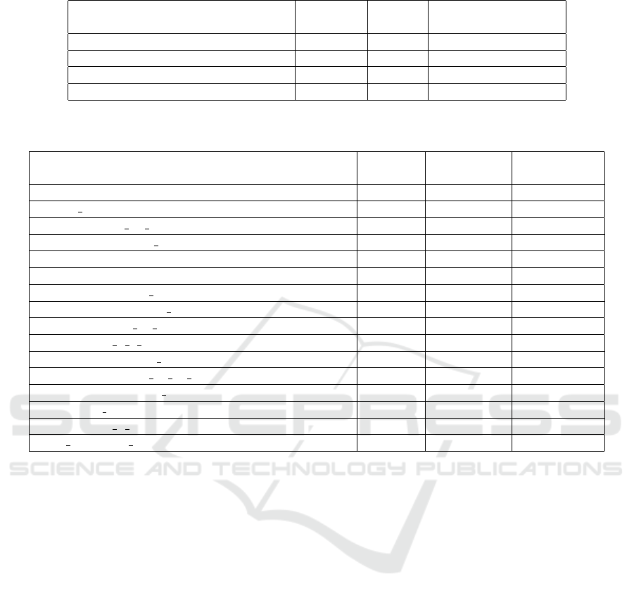
Table 1: Datasets Information.

Dataset Instances Classes

Avg Instances ± Std

per Class

Geo Images (Abel et al., 2019) 25725 45 571,67 ± 1290,90

Stanford Cars (Krause et al., 2013) 16185 196 84 ± 6,28

CIFAR-10 (Krizhevsky et al., 2009) 60000 10 6000 ± 0

STL10 (Coates et al., 2011) 100000 10 10000 ± 0

Table 2: Pre-trained Models Information. CNN indicates a convolutional neural networks architecture and Tr indicates a

transformer-based architecture.

Models

Output

Features

Parameters Architecture

alexnet(Krizhevsky, 2014) 256 61,100,840 CNN

clip rn50(He et al., 2016; Radford et al., 2021) 1024 63,000,000 CNN + Tr

clip vit b(Radford et al., 2021) 512 63,000,000 Tr + Tr

convnext large(Liu et al., 2022) 1536 197,767,336 CNN

densenet161(Huang et al., 2017) 2208 28,681,000 CNN

googlenet(Szegedy et al., 2015) 1000 6,624,904 CNN

inception v3(Szegedy et al., 2016) 1000 27,161,264 CNN

mnasnet1 3(Tan et al., 2019) 1000 6,282,256 CNN

mobilenet v3 large(Howard et al., 2019) 960 5,483,032 CNN

regnet y 3 2gf(Radosavovic et al., 2020) 1000 19,436,338 CNN

resnext101 64x4d(Xie et al., 2017) 1000 83,455,272 CNN

shufﬂenet v2 x2 0(Ma et al., 2018) 1000 7,393,996 CNN

squeezenet1 1(Iandola et al., 2016) 512 1,235,496 CNN

vgg19 bn(Simonyan and Zisserman, 2014) 512 143,678,248 CNN

vit h 14(Dosovitskiy et al., 2020) 1000 632,045,800 Tr

wide resnet101 2(Zagoruyko and Komodakis, 2016) 1000 126,886,696 CNN

3.3 Methodology

We aim to evaluate the performance of different avail-

able pre-trained models as feature extractors in the

image classiﬁcation task in other datasets. We used

the datasets and models previously detailed for con-

ducting our experiments. Notice also that since differ-

ent versions are available for each family of models,

we have selected a single model for each family that

presented the best overall performances according to

the literature.

Since we are considering 16 models and four

datasets, 64 experiments considering pairs of models

and datasets were performed.

In each experiment, each pre-trained model was

used as a feature extractor. Therefore, in this context,

all initial layers (except the last one) of the model, re-

sponsible for extracting relevant features from the in-

put images, were maintained, while the last layer was

replaced by a new classiﬁcation layer, with output size

N (where N is proportional to the number of classes

in the used dataset) using a linear activation function

and a softmax. During the training, the weights of

the initial layers (responsible for extracting features)

are kept frozen while the weights of the last layer are

adjusted.

For each experiment, the datasets went through

a homogeneous pre-processing. The pre-processing

consisted of applying resizing, center cropping, and

normalization. The resize is always done by decreas-

ing or increasing the size of the image’s smallest di-

mension to the size of the pre-trained model’s input.

Then, we perform the center crop, where the central

area of the image is cut as a square that matches the

size of the model’s input. Finally, we ensure that all

images are converted to RGB.

Each model was evaluated considering a 5-fold

cross-validation process. To comprehensively assess

the efﬁcacy of our approach, we adopted three differ-

ent metrics: accuracy, macro F1-score, and weighted

F1-score. These metrics offer a robust evaluation of

the results since they cover several evaluation aspects

in a multiclass classiﬁcation setting. Accuracy is a

fundamental measure of overall correctness (although

it can be misleading in contexts with data imbal-

ance), while the macro F1-score offers insights into

the model’s ability to perform effectively across all

classes, irrespective of class imbalances. Addition-

ICEIS 2024 - 26th International Conference on Enterprise Information Systems

468

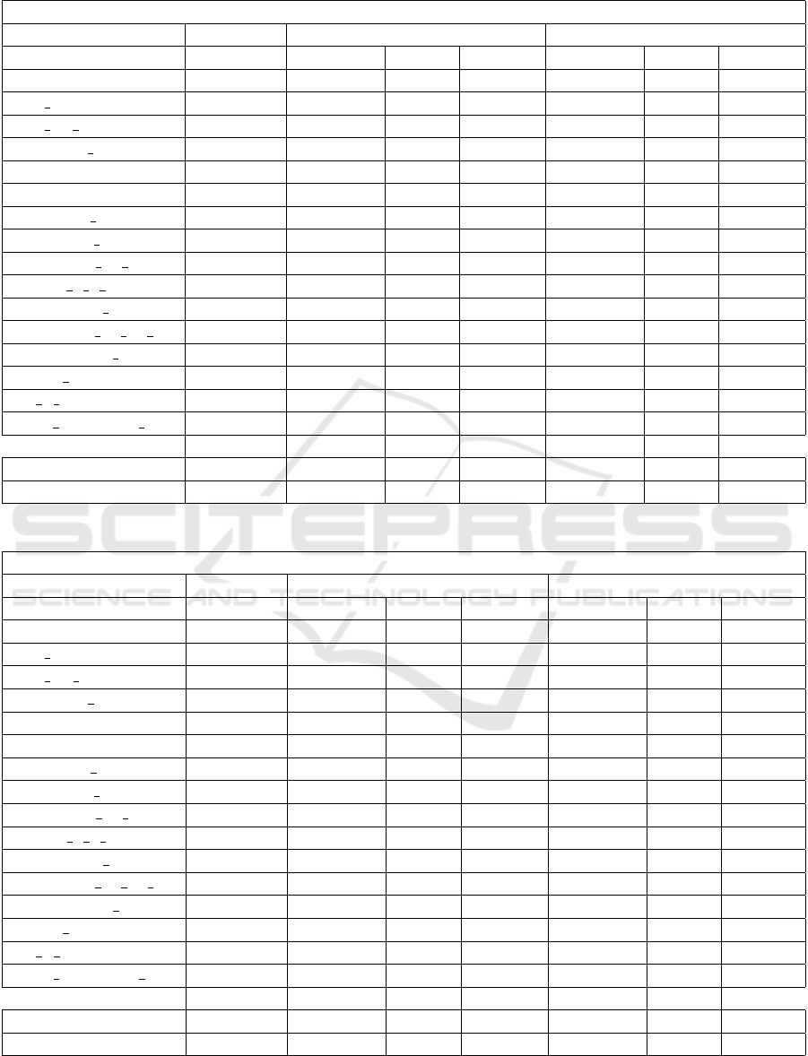
Table 3: Geological Images Dataset.

Geological Images Dataset

Macro Weighted

Model \Metrics Accuracy Precision Recall F-Score Precision Recall F-Score

alexnet 0,85 0,74 0,67 0,69 0,84 0,85 0,84

clip rn50 0,93 0,86 0,83 0,84 0,92 0,93 0,92

clip vit b 0,93 0,86 0,83 0,84 0,93 0,93 0,93

convnext large 0,91 0,84 0,80 0,82 0,91 0,91 0,91

densenet161 0,90 0,83 0,78 0,80 0,90 0,90 0,90

googlenet 0,87 0,75 0,72 0,73 0,86 0,87 0,86

inception v3 0,83 0,70 0,65 0,67 0,82 0,83 0,83

mnasnet1 3 0,88 0,77 0,73 0,75 0,87 0,88 0,87

mobilenet v3 large 0,90 0,82 0,77 0,79 0,90 0,90 0,90

regnet y 3 2gf 0,89 0,79 0,76 0,77 0,89 0,89 0,89

resnext101 64x4d 0,88 0,79 0,74 0,76 0,88 0,88 0,88

shufﬂenet v2 x2 0 0,89 0,80 0,76 0,78 0,89 0,89 0,89

squeezenet1 1 0,87 0,77 0,72 0,74 0,87 0,87 0,87

vgg19 bn 0,88 0,79 0,74 0,76 0,88 0,88 0,88

vit h 14 0,91 0,82 0,79 0,80 0,90 0,91 0,90

wide resnet101 2 0,89 0,79 0,75 0,77 0,89 0,89 0,89

Average 0,89 0,79 0,75 0,77 0,88 0,89 0,88

Standard Deviation 0,02 0,04 0,05 0,05 0,03 0,02 0,03

Table 4: Stanford Cars Dataset.

Stanford Cars Dataset

Macro Weighted

Model \Metrics Accuracy Precision Recall F-Score Precision Recall F-Score

alexnet 0,28 0,26 0,28 0,26 0,26 0,28 0,26

clip rn50 0,82 0,82 0,82 0,82 0,82 0,82 0,82

clip vit b 0,83 0,83 0,83 0,83 0,83 0,83 0,83

convnext large 0,65 0,65 0,64 0,64 0,65 0,65 0,64

densenet161 0,64 0,64 0,64 0,64 0,64 0,64 0,64

googlenet 0,41 0,41 0,41 0,41 0,40 0,41 0,40

inception v3 0,34 0,33 0,34 0,33 0,33 0,34 0,33

mnasnet1 3 0,42 0,42 0,42 0,42 0,41 0,42 0,41

mobilenet v3 large 0,56 0,56 0,56 0,55 0,56 0,56 0,55

regnet y 3 2gf 0,49 0,49 0,49 0,49 0,49 0,49 0,49

resnext101 64x4d 0,35 0,35 0,35 0,34 0,34 0,35 0,34

shufﬂenet v2 x2 0 0,50 0,50 0,50 0,50 0,50 0,50 0,50

squeezenet1 1 0,42 0,42 0,42 0,41 0,41 0,42 0,41

vgg19 bn 0,51 0,50 0,51 0,50 0,50 0,51 0,50

vit h 14 0,86 0,86 0,85 0,85 0,86 0,86 0,86

wide resnet101 2 0,44 0,44 0,44 0,44 0,44 0,44 0,44

Average 0,53 0,53 0,53 0,53 0,53 0,53 0,53

Standard Deviation 0,18 0,18 0,18 0,18 0,18 0,18 0,18

An Evaluation of Pre-Trained Models for Feature Extraction in Image Classiﬁcation

469

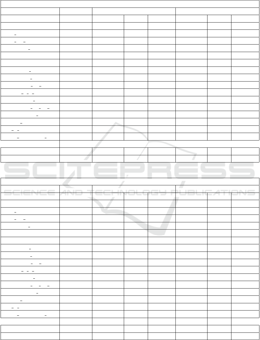
Table 5: CIFAR-10 Dataset.

CIFAR-10 Dataset

Macro Weighted

Model \Metrics Accuracy Precision Recall F-Score Precision Recall F-Score

alexnet 0,79 0,79 0,79 0,79 0,79 0,79 0,79

clip rn50 0,88 0,88 0,88 0,88 0,88 0,88 0,88

clip vit b 0,95 0,95 0,95 0,95 0,95 0,95 0,95

convnext large 0,96 0,96 0,96 0,96 0,96 0,96 0,96

densenet161 0,93 0,93 0,93 0,93 0,93 0,93 0,93

googlenet 0,87 0,87 0,87 0,87 0,87 0,87 0,87

inception v3 0,86 0,86 0,86 0,86 0,86 0,86 0,86

mnasnet1 3 0,90 0,90 0,90 0,90 0,90 0,90 0,90

mobilenet v3 large 0,91 0,91 0,91 0,91 0,91 0,91 0,91

regnet y 3 2gf 0,93 0,93 0,93 0,93 0,93 0,93 0,93

resnext101 64x4d 0,95 0,95 0,95 0,95 0,95 0,95 0,95

shufﬂenet v2 x2 0 0,92 0,92 0,92 0,92 0,92 0,92 0,92

squeezenet1 1 0,85 0,85 0,85 0,85 0,85 0,85 0,85

vgg19 bn 0,88 0,88 0,88 0,88 0,88 0,88 0,88

vit h 14 0,98 0,98 0,98 0,98 0,98 0,98 0,98

wide resnet101 2 0,95 0,95 0,95 0,95 0,95 0,95 0,95

Average 0,91 0,91 0,91 0,91 0,91 0,91 0,91

Standard Deviation 0,05 0,05 0,05 0,05 0,05 0,05 0,05

Table 6: STL10 Dataset.

STL10 Dataset

Macro Weighted

Model \Metrics Accuracy Precision Recall F-Score Precision Recall F-Score

alexnet 0,88 0,88 0,88 0,88 0,88 0,88 0,88

clip rn50 0,97 0,97 0,97 0,97 0,97 0,97 0,97

clip vit b 0,99 0,99 0,99 0,99 0,99 0,99 0,99

convnext large 0,99 0,99 0,99 0,99 0,99 0,99 0,99

densenet161 0,98 0,98 0,98 0,98 0,98 0,98 0,98

googlenet 0,96 0,96 0,96 0,96 0,96 0,96 0,96

inception v3 0,96 0,96 0,96 0,96 0,96 0,96 0,96

mnasnet1 3 0,97 0,97 0,97 0,97 0,97 0,97 0,97

mobilenet v3 large 0,96 0,96 0,96 0,96 0,96 0,96 0,96

regnet y 3 2gf 0,98 0,98 0,98 0,98 0,98 0,98 0,98

resnext101 64x4d 0,99 0,99 0,99 0,99 0,99 0,99 0,99

shufﬂenet v2 x2 0 0,97 0,97 0,97 0,97 0,97 0,97 0,97

squeezenet1 1 0,91 0,91 0,91 0,91 0,91 0,91 0,91

vgg19 bn 0,96 0,96 0,96 0,96 0,96 0,96 0,96

vit h 14 1,00 1,00 1,00 1,00 1,00 1,00 1,00

wide resnet101 2 0,99 0,99 0,99 0,99 0,99 0,99 0,99

Average 0,97 0,97 0,97 0,97 0,97 0,97 0,97

Standard Deviation 0,03 0,03 0,03 0,03 0,03 0,03 0,03

ICEIS 2024 - 26th International Conference on Enterprise Information Systems

470

ally, the weighted F1-score considers the non-uniform

distribution of classes, providing a nuanced under-

standing of performance weighted by class preva-

lence. The reported metrics are averages obtained

considering the performance in each test fold of this

cross-validation process.

Regarding the training hyperparameters, the

learning rate used in this study was 0.001 with a mo-

mentum of 0.9. We adopted the Adam optimizer with

default parameters, with the Cross-Entropy loss func-

tion. All executions were done using 100 epochs and

early stopping with a minimal improvement of 0.001

and patience of 5.

3.4 Results

The following tables represent the model’s perfor-

mance according to the selected metrics for each

dataset. Table 3 represents the model’s evaluation

on the Geological Images dataset. Table 4 repre-

sents the model’s evaluation according to Stanford

Cars dataset. Table 5 represents the model’s evalua-

tion considering the CIFAR-10 dataset. Table 6 repre-

sents the model’s evaluation for the STL10 dataset. In

each table, we highlight the model with the best per-

formance in green and with the lowest performance in

red.

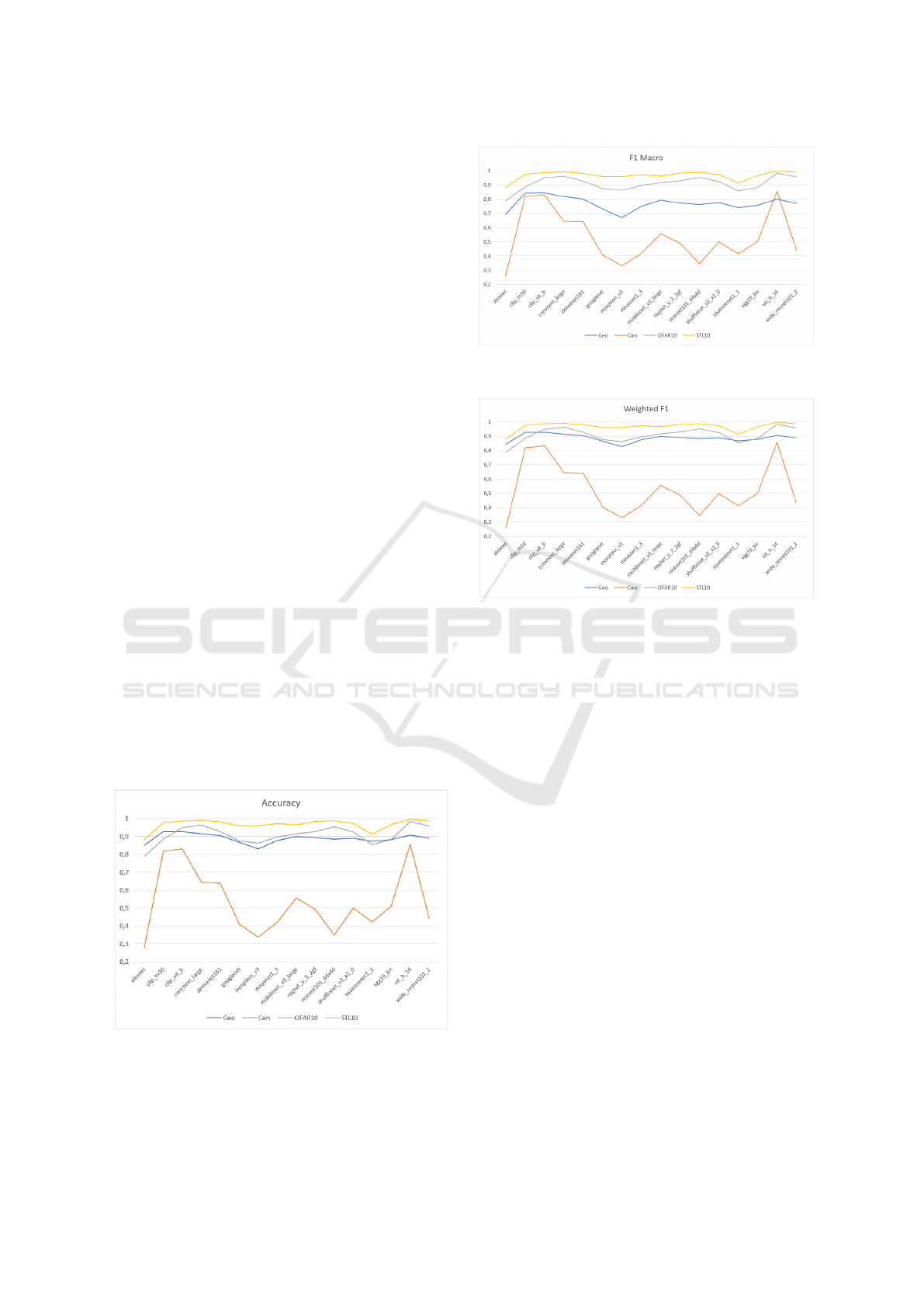
To facilitate the data analysis, we have represented

the results of our experiments in the following line

charts, demonstrating the performance (according to

different metrics) of each pre-trained model for classi-

fying the images in the four selected datasets. Figure

1 represents the accuracy, Figure 2 demonstrates the

macro f1-score, and Figure 3 indicates the weighted

f1-score of each model on each dataset.

Figure 1: Line chart representing the accuracy of each

model on each dataset.

The line charts in Figures 2-3 present a simi-

lar pattern of variation of the model’s performance

Figure 2: Line chart representing the macro f1-score of each

model on each dataset.

Figure 3: Line chart representing the weighted f1-score of

each model on each dataset.

across all datasets. We can also notice that, in gen-

eral, the model’s performance pattern increases, and

the differences among patterns decrease (resulting in

a smoother pattern) in the Geological Images dataset

when we consider the accuracy and the weighted av-

erages of the f1-score compared with the macro F1-

score. This behavior is expected since the imbalance

of this dataset is more apparent.

The CLIP-ViT-B and VisionTransformer-H/14

models generally show the best performances, con-

sidering all metrics in most datasets. The CLIP-ViT-

B presents the best performance in the Geological

Images dataset in all metrics. The CLIP-ResNet50

also performs well in the other datasets. However,

in the case of the CIFAR-10 and Geological Im-

ages datasets, this model’s performance is reasonably

lower than CLIP-ViT-B and ViT-H/14 in all metrics.

In the CIFAR-10 dataset, it is also worth highlight-

ing the good performance of ConvNeXt Large and

ResNeXt101-64x4D. The ConvNeXt Large model

also performs better than CLIP-ViT-B and CLIP-

ResNet50 in STL10.

In our evaluation, AlexNet presents the worst per-

formance on most datasets, considering all metrics.

This is expected since it is less sophisticated than

other models recently proposed. Inception V3 also

An Evaluation of Pre-Trained Models for Feature Extraction in Image Classiﬁcation

471

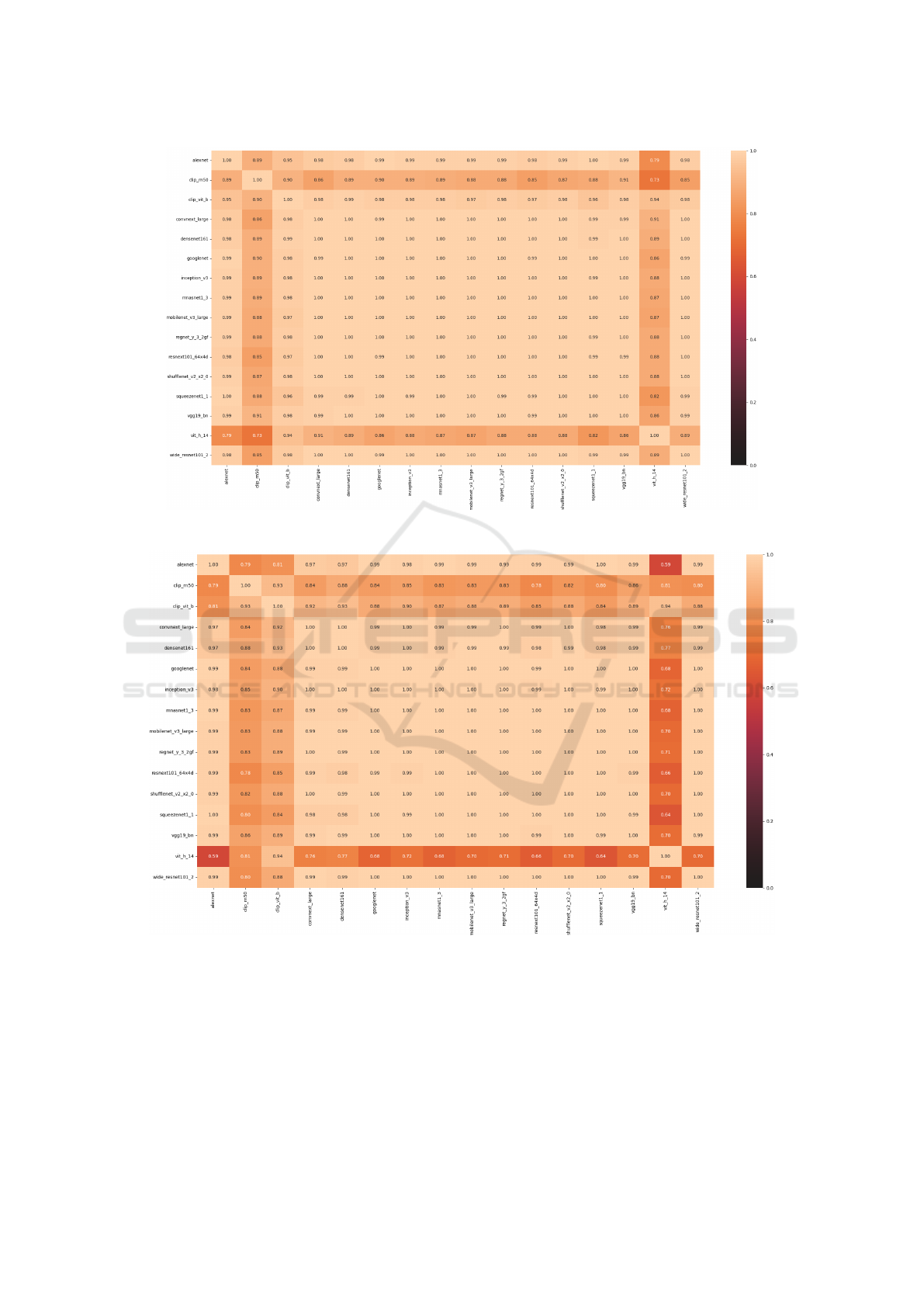
Figure 4: Heat map representing the correlation between each pair of models regarding accuracy.

Figure 5: Heat map representing the correlation between each pair of models regarding the macro f1-score.

performed poorly on the Stanford Cars, CIFAR-10,

and Geological Images datasets, where it performed

worst. Another model that had reasonably low perfor-

mance compared to the others was Squezenet1-1. The

poor performance of this model is more pronounced

on the CIFAR-10 and STL10 datasets.

The previous analysis (Figures 1-3) suggests that

some models present a very similar performance be-

havior across the datasets. In contrast, other models

exhibit behaviors that do not follow the general pat-

tern. To emphasize how similar are the model’s be-

haviors, we analyzed the Pearson correlation (Cohen

et al., 2009) of the performances of each pair of mod-

els across the datasets according to all the selected

metrics. The Figures 4-6 visually represent heat maps

with this information in a way that the darker a cell

ICEIS 2024 - 26th International Conference on Enterprise Information Systems

472

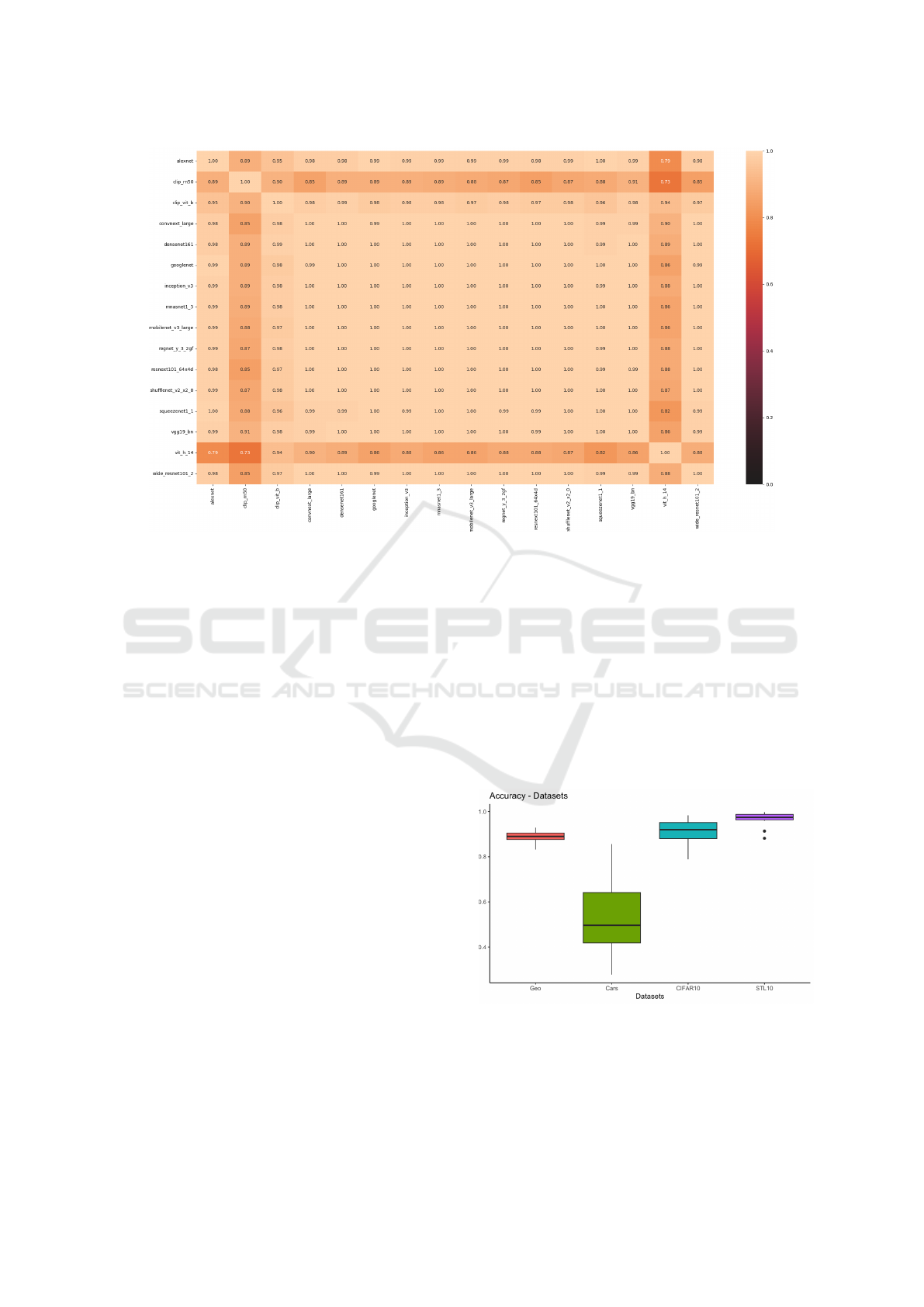
Figure 6: Heat map representing the correlation between each pair of models regarding the weighted f1-score.

gets corresponds to the lower the correlation of a

given pair of models, according to a given perfor-

mance metric. Figure 4 represents the pairwise Pear-

son correlation regarding the accuracy of each model,

Figure 5 represents the pairwise Pearson correlation

regarding the macro f1-score, and Figure 6 shows the

pairwise Pearson correlation regarding the weighted

f1-score between each pair of models.

Figures 4-6 suggest that the correlation of the per-

formances of each pair of models presents a similar

pattern in all metrics. We can also notice that, in all

performance metrics, the correlation between mod-

els based solely on CNN architectures is high (gen-

erally above 0.97). However, CLIP-ResNet50, CLIP-

ViT-B, and VisionTransformer-H/14 models present

a lower correlation with the performances of other

models solely based on CNN. In the case of CLIP-

ViT-B, the correlation with the other models is subtly

lower, considering accuracy and the weighted average

f1-score. However, this model’s correlation is signiﬁ-

cantly lower when we consider the macro average of

the f1-score. It is important to note that the CLIP-

ResNet50, CLIP-ViT-B, and VisionTransformer-H/14

models include transformers in their architectures.

This performance correlation analysis suggests that

this difference in the basic principles of the archi-

tecture of these models is correlated with this dif-

ference in the performance pattern of these mod-

els when compared to architectures based solely on

CNN. Further analysis should be done in the future

to investigate this hypothesis. The heat maps also

allow us to note that the correlations among CLIP-

ResNet50, CLIP-ViT-B, and VisionTransformer-H/14

models are low compared to the correlations among

the performances of models based solely on CNN.

In the previous analyses, we focused on the per-

formance of the models considered in our experi-

ments. In the following boxplots, we focused on an-

alyzing the datasets considered in our experiments.

Figure 7 represents the variation in accuracy. Figure

8 demonstrates the variation of macro f1-score. Fig-

ure 9 shows the variation of weighted f1-score in each

dataset.

Figure 7: Boxplot of accuracy for each dataset.

The boxplots present a similar pattern seen across

the different metrics. There are subtle differences

when comparing the macro average of the f1-score

with accuracy and weighted average. Note that, in

An Evaluation of Pre-Trained Models for Feature Extraction in Image Classiﬁcation

473

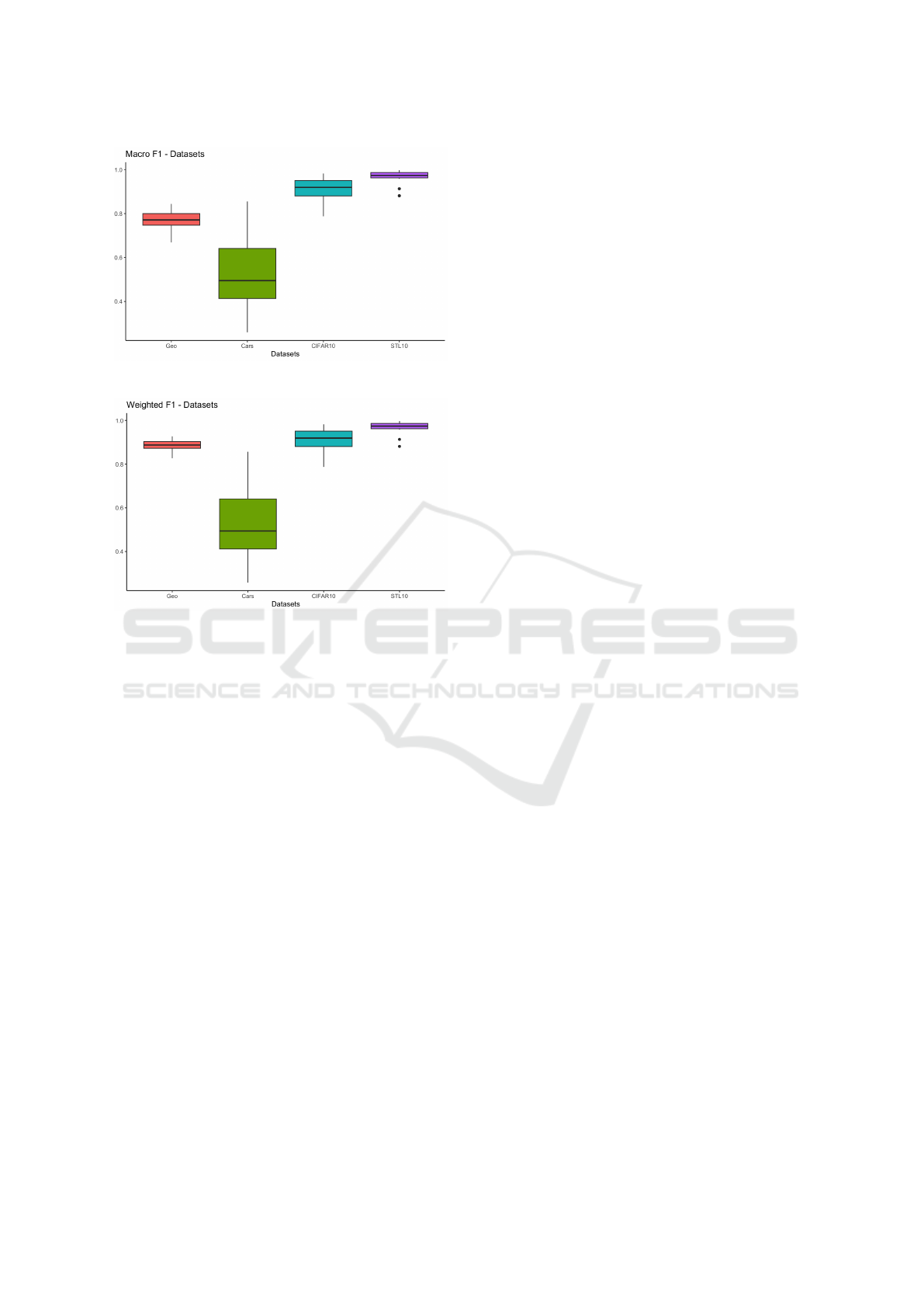
Figure 8: Boxplot of macro f1-score for each dataset.

Figure 9: Boxplot of weighted f1-score for each dataset.

general, the models tend to perform better in the

STL10 dataset; in second place, CIFAR-10 has the

best overall results; in third place, the dataset of

Geological Images and, ﬁnally, the dataset with the

worst performances in general, is the Stanford Cars.

The low performance in the Stanfor cars is expected

since this dataset has a large number of classes, few

samples per class, and includes images with differ-

ent sizes and features at different scales. The Geo-

logical Images dataset has similar properties but has

fewer classes and more samples per class than Stan-

ford Cars, although it presents a more signiﬁcant im-

balance. These charts allow us to conclude that the

Stanford Cars dataset is the most challenging among

those analyzed, with the worst and most considerable

variability of performances in all metrics. Besides

that, we can also notice that the STL10 dataset and

Geological Images have a smaller variability in the

performance of the different models when compared

with the other two datasets.

4 CONCLUSION

In this work, our goal was to compare the perfor-

mance of sixteen pre-trained neural networks for fea-

ture extraction in four different datasets. By analyz-

ing the accuracy and macro and weighted averages

of the f1-score in our experiments and considering

all the datasets, our experiments suggest that CLIP-

ViT-B and VisionTransformer-H/14 achieved the best

performance results. Besides that, CLIP-ResNet50

achieved performance similar to the performance

achieved by CLIP-ViT-B and VisionTransformer-

H/14 and even lower variability. It is important to no-

tice that CLIP-ViT-B, VisionTransformer-H/14, and

CLIP-ResNet50 include transformers in their archi-

tectures. Thus, our results suggest that the principles

underlying the transformers can be the reason cor-

roborating these remarkable results, but with further

studies, we can investigate this hypothesis.

Among the CNN-based architectures, ConvNeXt

Large presents the best performance, in general, and

lower variability when compared to other CNN-based

architectures. AlexNet showed the worst performance

and high variability. Besides that, ResNeXt101-

64x4D, Wide ResNet 101-2, and Inception V3 also

showed high variability.

Our analysis also showed that the performances

of models based solely on CNN architectures present

a high Pearson correlation in all performance met-

rics. However, the performances of CLIP-ResNet50,

CLIP-ViT-B, and VisionTransformer-H/14 models

show a lower correlation with other models based

solely on CNN. We can hypothesize that this differ-

ence is due to differences regarding the basic prin-

ciples of the architecture of these models. How-

ever, the correlations among CLIP-ResNet50, CLIP-

ViT-B, and VisionTransformer-H/14 models are low

compared to correlations among the performances of

CNN-based models. Further studies are needed to in-

vestigate this ﬁnding better.

Our analysis also has shown that the selected mod-

els performed better on the STL10 dataset, followed

by CIFAR-10, then the Geological Images dataset,

and ﬁnally, the Stanford Cars dataset. Thus, the Stan-

ford Cars dataset is the most challenging dataset eval-

uated in this work. The Stanford Cars present a con-

siderable image size (compared with CIFAR-10 and

STL10, for example) and many classes with just a few

samples per class. These characteristics may explain

this result. The Geological Images dataset shares

some of the properties of the Stanford Cars dataset.

Still, it presents fewer classes and has more images

per class, in general.

The investigation presented in this work can pro-

vide evidence supporting the choice of transfer learn-

ing models in image classiﬁcation tasks in “real-

world” datasets such as the geological dataset. Since

our evaluation also covered other image datasets with

ICEIS 2024 - 26th International Conference on Enterprise Information Systems

474

different characteristics, it can suggest reasonable

model choices in other domains.

In future works, it is important to expand the anal-

ysis by including other image datasets to make the

analysis more comprehensive. Besides that, the in-

vestigation can also be expanded to include more pre-

trained models that eventually were not considered in

the scope of this work. Furthermore, future works

could also investigate the relationship between the un-

derlying principles of each architecture, the properties

of the datasets used in the pre-training of these mod-

els, and the properties of the target datasets in which

the pre-trained models are applied to extract features.

This investigation can reveal insights into what makes

the pre-trained model best suited for each task.

ACKNOWLEDGMENTS

The authors would like to thank the Brazilian Na-

tional Council for Scientiﬁc and Technological Devel-

opment (CNPq) and Petrobras for the ﬁnancial sup-

port of this work.

REFERENCES

Abel, M., Gastal, E. S. L., Michelin, C. R. L., Maggi, L. G.,

Firnkes, B. E., Pachas, F. E. H., and dos Santos Al-

varenga, R. (2019). A knowledge organization system

for image classiﬁcation and retrieval in petroleum ex-

ploration domain. In ONTOBRAS.

Abou Baker, N., Zengeler, N., and Handmann (2022).

Uwe. a transfer learning evaluation of deep neural net-

works for image classiﬁcation. Machine Learning and

Knowledge Extraction, 4(1):22–41.

Alzubaidi, L. et al. (2021). Review of deep learning: Con-

cepts, cnn architectures, challenges, applications, fu-

ture directions. Journal of big Data, 8(1):1–74.

Arslan, Y., Allix, K., Veiber, L., Lothritz, C., Bissyand

T. F., Klein, J., and Goujon, A. (2021). A compari-

son of pre-trained language models for multi-class text

classiﬁcation in the ﬁnancial domain. In Companion

Proceedings of the Web Conference 2021, pages 260–

268.

Coates, A., Ng, A., and Lee, H. (2011). An analy-

sis of single-layer networks in unsupervised feature

learning. In Proceedings of the fourteenth interna-

tional conference on artiﬁcial intelligence and statis-

tics, pages 215–223. JMLR Workshop and Confer-

ence Proceedings.

Cohen, I., Huang, Y., Chen, J., Benesty, J., Benesty, J.,

Chen, J., Huang, Y., and Cohen, I. (2009). Pearson

correlation coefﬁcient. Noise reduction in speech pro-

cessing, pages 1–4.

De Lima, R. P. et al. (2019). Deep convolutional neural

networks as a geological image classiﬁcation tool. The

Sedimentary Record, 17(2):4–9.

Deng, J., Dong, W., Socher, R., Li, L.-J., Li, K., and Fei-

Fei, L. (2009). Imagenet: A large-scale hierarchical

image database. In 2009 IEEE conference on com-

puter vision and pattern recognition, pages 248–255.

Ieee.

Dosovitskiy, A., Beyer, L., Kolesnikov, A., Weissenborn,

D., Zhai, X., Unterthiner, T., Dehghani, M., Minderer,

M., Heigold, G., Gelly, S., et al. (2020). An image is

worth 16x16 words: Transformers for image recogni-

tion at scale. arXiv preprint arXiv:2010.11929.

Fawaz, H. I. et al. (2018). Transfer learning for time series

classiﬁcation. In 2018 IEEE international conference

on big data (Big Data), pages 1367–1376. IEEE p.

He, K. et al. (2016). Deep residual learning for image

recognition. In Proceedings of the IEEE conference

on computer vision and pattern recognition p, pages

770–778.

Hollink, L., Schreiber, G., Wielemaker, J., Wielinga, B.,

et al. (2003). Semantic annotation of image collec-

tions. In Knowledge capture, volume 2.

Howard, A., Sandler, M., Chu, G., Chen, L.-C., Chen, B.,

Tan, M., Wang, W., Zhu, Y., Pang, R., Vasudevan, V.,

et al. (2019). Searching for mobilenetv3. In Pro-

ceedings of the IEEE/CVF international conference

on computer vision, pages 1314–1324.

Huang, G., Liu, Z., Van Der Maaten, L., and Weinberger,

K. Q. (2017). Densely connected convolutional net-

works. In Proceedings of the IEEE conference on

computer vision and pattern recognition, pages 4700–

4708.

Iandola, F. N., Han, S., Moskewicz, M. W., Ashraf, K.,

Dally, W. J., and Keutzer, K. (2016). Squeezenet:

Alexnet-level accuracy with 50x fewer parame-

ters and¡ 0.5 mb model size. arXiv preprint

arXiv:1602.07360.

Karpatne, A. et al. (2018). Machine learning for the

geosciences: Challenges and opportunities. IEEE

Transactions on Knowledge and Data Engineering,

31(8):1544–1554.

Kieffer, B., Babaie, M., Kalra, S., and Tizhoosh,

H. R. (2017). Convolutional neural networks for

histopathology image classiﬁcation: Training vs. us-

ing pre-trained networks. In 2017 Seventh Interna-

tional Conference on Image Processing Theory, Tools

and Applications (IPTA), pages 1–6. IEEE.

Krause, J., Stark, M., Deng, J., and Fei-Fei, L. (2013). 3d

object representations for ﬁne-grained categorization.

In 4th International IEEE Workshop on 3D Represen-

tation and Recognition (3dRR-13), Sydney, Australia.

Krizhevsky, A. (2014). One weird trick for paralleliz-

ing convolutional neural networks. arXiv preprint

arXiv:1404.5997.

Krizhevsky, A., Hinton, G., et al. (2009). Learning multiple

layers of features from tiny images.

Kumar, J. S., Anuar, S., and Hassan, N. H. (2022). Trans-

fer learning based performance comparison of the pre-

trained deep neural networks. International Journal of

Advanced Computer Science and Applications, 13:1.

An Evaluation of Pre-Trained Models for Feature Extraction in Image Classiﬁcation

475

Lanchantin, J., Wang, T., Ordonez, V., and Qi, Y. (2021).

General multi-label image classiﬁcation with trans-

formers. In Proceedings of the IEEE/CVF Conference

on Computer Vision and Pattern Recognition (CVPR),

pages 16478–16488.

Liu, Z., Mao, H., Wu, C.-Y., Feichtenhofer, C., Darrell, T.,

and Xie, S. (2022). A convnet for the 2020s. In Pro-

ceedings of the IEEE/CVF Conference on Computer

Vision and Pattern Recognition, pages 11976–11986.

Lumini, A. and Nanni, L. (2019). Deep learning and trans-

fer learning features for plankton classiﬁcation. Eco-

logical informatics, 51:33–43.

Ma, N., Zhang, X., Zheng, H.-T., and Sun, J. (2018). Shuf-

ﬂenet v2: Practical guidelines for efﬁcient cnn archi-

tecture design. In Proceedings of the European con-

ference on computer vision (ECCV), pages 116–131.

Mallouh, A. A., Qawaqneh, Z., and Barkana, B. D.

(2019). Utilizing cnns and transfer learning of pre-

trained models for age range classiﬁcation from un-

constrained face images. Image and Vision Comput-

ing, 88:41–51.

Maniar, H. et al. (2018). Machine-learning methods in geo-

science. In 2018 SEG International Exposition and

Annual Meeting. OnePetro.

Mormont, R., Geurts, P., and Mar

ee, R. (2018). Comparison

of deep transfer learning strategies for digital pathol-

ogy. In Proceedings of the IEEE conference on com-

puter vision and pattern recognition workshops, pages

2262–2271.

Pferd, J. (2010). The challenges of integrating structured

and unstructured data. In 14th Petroleum Network Ed-

ucation Conference. s.n, S.l.

Radford, A., Kim, J. W., Hallacy, C., Ramesh, A., Goh, G.,

Agarwal, S., Sastry, G., Askell, A., Mishkin, P., Clark,

J., et al. (2021). Learning transferable visual models

from natural language supervision. In International

conference on machine learning, pages 8748–8763.

PMLR.

Radosavovic, I., Kosaraju, R. P., Girshick, R., He, K., and

Doll

ar, P. (2020). Designing network design spaces.

In Proceedings of the IEEE/CVF conference on com-

puter vision and pattern recognition, pages 10428–

10436.

Simonyan, K. and Zisserman, A. (2014). Very deep con-

volutional networks for large-scale image recognition.

arXiv preprint arXiv:1409.1556.

Sun, H. et al. (2021). Convolutional neural networks

based remote sensing scene classiﬁcation under clear

and cloudy environments. In Proceedings of the

IEEE/CVF International Conference on Computer Vi-

sion p, pages 713–720.

Szegedy, C., Liu, W., Jia, Y., Sermanet, P., Reed, S.,

Anguelov, D., Erhan, D., Vanhoucke, V., and Rabi-

novich, A. (2015). Going deeper with convolutions.

In Proceedings of the IEEE conference on computer

vision and pattern recognition, pages 1–9.

Szegedy, C., Vanhoucke, V., Ioffe, S., Shlens, J., and Wo-

jna, Z. (2016). Rethinking the inception architecture

for computer vision. In Proceedings of the IEEE con-

ference on computer vision and pattern recognition,

pages 2818–2826.

Tan, M., Chen, B., Pang, R., Vasudevan, V., Sandler, M.,

Howard, A., and Le, Q. V. (2019). Mnasnet: Platform-

aware neural architecture search for mobile. In Pro-

ceedings of the IEEE/CVF conference on computer vi-

sion and pattern recognition, pages 2820–2828.

Todescato, M. V., Garcia, L. F., Balreira, D. G., and Carbon-

era, J. L. (2023). Multiscale context features for geo-

logical image classiﬁcation. In Filipe, J., Smialek, M.,

Brodsky, A., and Hammoudi, S., editors, Proceedings

of the 25th International Conference on Enterprise In-

formation Systems, ICEIS 2023, Volume 1, Prague,

Czech Republic, April 24-26, 2023, pages 407–418.

SCITEPRESS.

Todescato, M. V., Garcia, L. F., Balreira, D. G., and Car-

bonera, J. L. (2024). Multiscale patch-based feature

graphs for image classiﬁcation. Expert Systems with

Applications, 235:121116.

Xie, S., Girshick, R., Doll

ar, P., Tu, Z., and He, K. (2017).

Aggregated residual transformations for deep neural

networks. In Proceedings of the IEEE conference on

computer vision and pattern recognition, pages 1492–

1500.

Zagoruyko, S. and Komodakis, N. (2016). Wide residual

networks. arXiv preprint arXiv:1605.07146.

ICEIS 2024 - 26th International Conference on Enterprise Information Systems

476