A Computer Vision-Based Method for Collecting Ground Truth for

Mobile Robot Odometry

Ricardo C. C

amara de M. Santos

, Mateus Coelho Silva

and Ricardo A. R. Oliveira

Departmento de Computac¸

ao - DECOM, Universidade Federal de Ouro Preto - UFOP, Ouro Preto, Brazil

Keywords:

Odometry, Mobile Robots, Odometry Database, Odometry Calibration.

Abstract:

With the advancement of artiﬁcial intelligence and embedded hardware development, the utilization of various

autonomous navigation methods for mobile robots has become increasingly feasible. Consequently, the need

for robust validation methodologies for these locomotion methods has arisen. This paper presents a novel

ground truth positioning collection method relying on computer vision. In this method, a camera is positioned

overhead to detect the robot’s position through a computer vision technique. The image used to retrieve the

positioning ground truth is collected synchronously with data from other sensors. By considering the camera-

derived position as the ground truth, a comparative analysis can be conducted to develop, analyze, and test

different robot odometry methods. In addition to proposing the ground truth collection methodology in this

article, we also compare using a DNN to perform odometry using data from different sensors as input. The

results demonstrate the efﬁcacy of our ground truth collection method in assessing and comparing different

odometry methods for mobile robots. This research contributes to the ﬁeld of mobile robotics by offering a

reliable and versatile approach to assess and compare odometry techniques, which is crucial for developing

and deploying autonomous robotic systems.

1 INTRODUCTION

Mobile robotics is a technology and research area that

has gained much attention recently. This increase in

attention given to these robots is due to the variety of

areas in which they can be used, such as transporta-

tion, cleaning services, surveillance, search, and res-

cue, among others (Alatise and Hancke, 2020).

An autonomous mobile robot can move around its

assigned environment (an industrial plant, laboratory,

mine, and others) without human intervention. A mo-

bile robot is divided into four main tasks: locomotion,

perception, cognition, and navigation (Rubio et al.,

2019). Locomotion is responsible for the movement

of the robot in the environment. For this matter, it

is necessary to understand the environment, the loco-

motion mechanism (wheels, conveyors, legs, among

others), its dynamics, and control theory. Perception

refers to sensing to obtain information from the envi-

ronment and the robot itself. Cognition is responsible

for analyzing the data acquired in perception, creat-

https://orcid.org/0000-0002-2058-6163

https://orcid.org/0000-0003-3717-1906

https://orcid.org/0000-0001-5167-1523

ing a representation of the environment, and planning

the actions to be taken. Navigation is the most im-

portant and most challenging task of an autonomous

robot, and its objective is to move the robot from one

location in the environment to another. This task in-

volves computing a collision-free trajectory and mov-

ing along this trajectory (Niloy et al., 2021).

One of the most critical challenges in carrying out

navigation is self-localization, which consists of de-

termining the location and orientation of the robot at

each instant of time throughout its operation. Only

with self-location is it possible for the robot to navi-

gate autonomously in a given environment. The tradi-

tional localization technique that is most used on au-

tonomous platforms is the Global Positioning System

(GPS). It is a global satellite system that uses a radio

system to determine the position and speed of mov-

ing objects (Srinivas and Kumar, 2017). Although

the most advanced GPS systems can provide position-

ing, at best, with centimeter accuracy, they are still

not reliable enough for autonomous navigation plat-

forms, especially in conﬁned, aquatic, underground,

and aerial environments (Srinivas and Kumar, 2017).

In the last decade, many techniques have emerged

featuring Simultaneous Localization and Mapping

116

Santos, R., Silva, M. and Oliveira, R.

A Computer Vision-Based Method for Collecting Ground Truth for Mobile Robot Odometry.

DOI: 10.5220/0012622900003690

Paper published under CC license (CC BY-NC-ND 4.0)

In Proceedings of the 26th International Conference on Enterprise Information Systems (ICEIS 2024) - Volume 1, pages 116-127

ISBN: 978-989-758-692-7; ISSN: 2184-4992

(SLAM) methods (Mur-Artal et al., 2015),(Khan

et al., 2021). These techniques focus on calculating

the position and orientation of robots based on data

obtained from their own sensors, as opposed to the

use of external sensors such as GPS. In this way, they

are based on odometry for positioning and navigation.

Odometry is the use of motion sensors to determine

the change in position of the robot in relation to a pre-

viously known position.

This work presents a methodology based on com-

puter vision for positioning ground truth collection to

validate, calibrate, and compare odometry techniques

for mobile robots. In this method, a camera is po-

sitioned above the area where the robot will move.

Markings are used in this location and on the robot,

which is later detected by processing the camera im-

age. A transformation is applied to the camera im-

age to map the image in an orthogonal environment,

thus creating a Cartesian plane where the detection

of the marking tag positioned on the robot informs

us of its positioning and orientation. Data collection

from sensors, together with the capture of each im-

age, must be carried out. This way, it is possible to

calculate the error of the odometry method used. By

calculating the error of several methods, a comparison

can be made between them. Through this methodol-

ogy, it is also possible to generate a database to create

new methods using the desired sensors. In addition

to proposing this ground truth collection method, this

work also compares the use of different sensors and

combinations between them and applies DNNs to per-

form odometry.

2 THEORETICAL REFERENCES

Before presenting the ground truth collection method-

ology proposed in this study, it is essential to intro-

duce some principles that underlie this work. In this

section, the essential theoretical foundations for the

development of the methodology we are proposing

and for the execution of the experiments are outlined.

2.1 Mobile Robots

First, we must present the concept of mobile robotics.

Although there is no generally accepted deﬁnition for

the term ”mobile robot,” it is often understood as a de-

vice capable of moving autonomously from one place

to another to achieve a set of objectives (Tzafestas,

2013). An autonomous mobile robot (AMR) is de-

signed to perform continuous navigation while avoid-

ing collisions with obstacles in a speciﬁc environment

(Ishikawa, 1991). The AMR is designed to require lit-

tle or no human intervention during its navigation and

locomotion, being able to follow a predeﬁned trajec-

tory both indoors and outdoors.

The fundamental principles of mobile robotics

cover the following tasks: locomotion, perception,

cognition, and navigation. In indoor environments,

the mobile robot commonly relies on elements such

as ﬂoor mapping, sonar location, and the inertial mea-

surement unit (IMU), among other sensors. The robot

must be equipped with several sensors capable of pro-

viding an internal representation of the environment

to ensure its functioning. These sensors can be in-

corporated directly into the robot or play the role of

external sensors positioned in different locations in

the environment, transmitting the collected informa-

tion to the robot.

2.2 Odometry

Odometry measures distance and is a fundamental

method used by robots for navigation (Ben-Ari et al.,

2018). Therefore, odometry is essential to estimate

the position and orientation of a mobile robot based

on the measurement variation of the robot’s sensors.

Generally, odometry uses data on the relative move-

ment of the wheels, such as rotation and distance trav-

eled, to calculate the trajectory traveled by the robot.

Although it is a very valid way to estimate the robot’s

position, odometry can suffer from the accumulation

of errors over time.

As the positioning measurement is based on the

distance traveled, each error in the distance traveled

will accumulate over time. These errors can occur for

several reasons, such as inaccuracies in sensor mea-

surements and variable environmental conditions. A

variety of odometry techniques can be adopted, such

as visual odometry using cameras (Nist

er et al., 2004),

odometry with lidar (Wang et al., 2021), among oth-

ers, and sensor fusion can also be applied to have

more robust odometry.

2.3 Ground Truth

Ground truth is an essential concept in several areas,

including machine learning. Refers to a set of data

that accurately represents phenomena, situations, or

measurements of magnitudes. For example, to eval-

uate the positioning of a robot, we can collect its

actual positions using reliable measurement methods

and compare these positions with those generated by

the method we intend to implement or evaluate. Thus,

the positions considered real are our ground truth. A

reliable ground truth is crucial for validating and eval-

uating algorithms, providing a solid basis for analyz-

A Computer Vision-Based Method for Collecting Ground Truth for Mobile Robot Odometry

117

ing and improving them. In summary, ground truth

is a fundamental concept to guarantee the accuracy

and reliability of approaches in various scientiﬁc and

technological areas.

2.4 Thin Plate SPlines

The term ’spline’ refers to a craftsman’s tool, a thin,

ﬂexible strip of wood or metal used to trace smooth

curves. Various weights would be applied in various

positions so that the strip would bend according to

their number and position. These positions would be

forced through a set of ﬁxed points: metal pins, the

ribs of a boat, and others. On a ﬂat surface, these

weights often had a hook attached and were easy to

manipulate. The shape of the folded material would

naturally take the form of a spline curve.

Similarly, splines are used in statistics to re-

produce ﬂexible shapes mathematically. Nodes are

placed at various places within the data range to iden-

tify the points where adjacent functional parts come

together. Instead of metal or wood strips, smooth

functional pieces (usually low-order polynomials) are

chosen to ﬁt the data between two consecutive nodes.

The type of polynomial and the number and position

of nodes deﬁne the type of spline (Perperoglou et al.,

2019).

For understanding purposes, consider an exam-

ple of a cubic spline. Given a set of control points

, y

), (x

, y

), ..., (x

, y

) and you want to ﬁt a cubic

spline to these points. The general form of a cubic

spline between two points x

and x

i+1

is given by the

Equation 1:

(x) = a

+ b

(x − x

) + c

(x − x

)

+ d

(x − x

)

(1)

where:

• a

, b

, c

, d

: are coefﬁcients that need to be deter-

mined for each segment i

• x

: is the starting point of the segment

• x

i+1

: is the end point of the segment

These coefﬁcients are determined so that the

spline is smooth and passes through the control

points.

Then for each segment i, you have a set of condi-

tions based on the control points.

• S

) = y

• S

i+1

) = y

i+1

• S

′

) = S

′

i−1

)

• S

′′

) = S

′′

i−1

)

The ﬁrst two conditions guarantee that they start

and end by passing checkpoints. The last two con-

ditions guarantee that the estimated curve passes

smoothly through the points. This is because the ﬁrst

derivative represents the slope of the curve and the

second the concavity.

The Thin Plate Spline (TPS) is a speciﬁc spline

used in interpolation and surface adjustment (Duchon,

1977). TPS is used in problems where surface

smoothness is required, such as deformation mapping

(Donato and Belongie, 2002), three-dimensional re-

construction (Sokolov et al., 2017), and other image

processing applications (Atik et al., 2020).

The spline function that minimizes the curvature

of a plane is given by the Equation 2:

f (x, y) = a + bx + cy +

∑

i=1

U(r) (2)

where:

• a, b, c and w

(i = 1, ..., n): spline coefﬁcients

• U: radial basis function

• r: distance from point x, y to control point (x

, y

)

The basis of the TPS formulation is the radial ba-

sis function U, given by the Equation 3:

U(r) = r

log(r) (3)

3 RELATED WORKS

Odometry implementation is directly related to data

collection, where the collected data are used to test,

calibrate, and compare odometry methods. Thus, we

reviewed works on data collection focusing on the en-

vironment, using sensors and ground truth estimation

methods, which we will discuss in this section.

In (Kirsanov et al., 2019), DISCOMAN is pre-

sented: a database for odometry, mapping, and nav-

igation of mobile robots. In addition to this data, they

also offer a ground truth for semantic image segmen-

tation. The database was generated using image ren-

dering of 3D environments based on realistic lighting

models and simulating the behavior of a smart robot

exploring houses. The data was obtained from simu-

lations in a digital environment of original residential

layouts created for renovations of real houses. The

authors synthesized realistic trajectories and rendered

image sequences. They generated 200 sequences that

included between 3000 and 5000 data samples each.

The data collected were RGB images, depth, IMU,

and house occupancy grid.

In the work shown in (Chen et al., 2018), the

Oxford Inertial Odometry Dataset (OxIOD) database

ICEIS 2024 - 26th International Conference on Enterprise Information Systems

118

for inertial odometry was presented, with IMU and

magnetometer data in 158 sequences and a total dis-

placement of 42.587 km. The data collected in this

database were generated through simulation of every-

day activities in indoor environments. Location la-

bels, speeds, and orientations were generated using

an optical motion capture system named Vicon for

data collection in a single room. For sequences at

larger locations, Google Tango’s inertial visual odom-

etry tracker was used to provide approximate infor-

mation. Data was collected from different users and

devices, with varying movements and locations of de-

vice positioning, such as a backpack, pocket, holding

in hand, and above a cart.

The authors of (Cort

es et al., 2018) presented

a database for inertial visual odometry and SLAM.

They built a device combining an iPhone 6, a Google

Pixel Android phone, and a Google Tango device to

do this. With the iPhone 6, they collected video, GPS,

Barometer, gyroscope, accelerometer, magnetometer,

and position and orientation data using the ARKit

SDK. Position and orientation data were collected us-

ing the ARCore SDK with the Google Pixel. With

Google Tango, position and orientation, wide-angle

camera video, and point cloud were collected. The

ground truth was generated through the use of purely

inertial odometry and the use of ﬁxed points of known

positions. The collected data sequences contain about

4.5 kilometers of unrestricted movement in various

indoor and outdoor environments, such as streets, of-

ﬁces, shopping malls, subways, and campuses.

In (Ramezani et al., 2020), The Newer College

Dataset database is presented to us, with depth, in-

ertial, and visual data collection. Data was collected

using a portable device carried manually at typical

walking speeds for almost 2.2km around New Col-

lege, Oxford. The handheld device comprises a 3D

LiDAR and a stereo camera. Both the camera and

the LIDAR have an independent IMU. This database

includes the internal environment (built area), the ex-

ternal environment (open spaces), and areas with veg-

etation. The ground truth was generated using a sec-

ond high-precision LIDAR, the BLK360, with an ac-

curacy of approximately 3 cm.

In (Gurturk et al., 2021), the authors bring a

database for visual inertial odometry called the YTU

database. The dataset was collected at Yildiz Tech-

nical University (YTU) in an outdoor area by an ac-

quisition system mounted on a ground vehicle, a van.

The acquisition system includes two GoPro Hero 7

cameras, an Xsens MTi-G-700 IMU, and two Topcon

HyperPro GPS receivers. All these sensors were posi-

tioned on top of the van and used to acquire data along

a trajectory of 535 meters in the Yıldız Technical Uni-

versity ﬁeld. The total duration of data collection was

2 minutes. The ground truth was generated using GPS

positioning.

The work (Carlevaris-Bianco et al., 2016) shows a

database for autonomous robots collected at the Uni-

versity of Michigan. The collected dataset consists

of omnidirectional imagery, 3D lidar, planar lidar,

GPS, GNSS RTK, IMU, and ﬁber optic gyroscope.

All these sensors were installed on a Segway robot.

This database is focused on long-term data collec-

tion in changing environments. Therefore, data were

collected in 27 sessions with approximately 15 days

between each collection over 15 months. The data

collection sessions took place on the University of

Michigan campus, both outdoors and indoors, with

varied trajectories, different times of the day, and dif-

ferent seasons. The ground truth was generated using

SLAM algorithms and GPS RTK.

In (Peynot et al., 2010), the Marulan database is

shown, which aims to collect data in an external en-

vironment using a wheeled robot, in this case, an

ARGO platform. Data were collected from four 2D

laser scanners with a 180º ﬁeld of view, radar, a color

camera, and an infrared camera. Data saving was

done synchronously. The collection was carried out

in an environment with a stationary and moving robot

with static objects with prior positioning. The ground

truth was done manually by measuring the geometry

and positioning of objects at the collection site. Data

was collected under controlled environmental condi-

tions, including dust, smoke, and rain. Forty collec-

tion sessions were carried out, generating 400GB of

data.

In (Ceriani et al., 2009), a similar approach to ours

is shown. This paper presents two ground truth col-

lection techniques for indoor environments. These

techniques are based on a network of ﬁxed cam-

eras and ﬁxed laser scanners. The techniques were

named GTVision and GTLaser, respectively. In the

GTLaser technique, the robot’s positioning is recon-

structed based on a rectangular shell attached to the

robot. In GTVision, the robot’s pose is reconstructed

based on observing a set of visual markers attached to

the robot. The relative position of the markers on the

robot was previously calculated using a portable cam-

era, and the three-dimensional rigid transformations

that relate each marker to the robot’s position were

estimated. During collection, the robot’s position is

estimated by detecting markers and applying 3D rigid

transformations. The GTLaser technique is used for

2D positioning detection, and GTVision is used for

3D positioning detection. The GTLaser is necessary

to align the lasers and calculate the relative position-

ing between them, in addition to ensuring that there

A Computer Vision-Based Method for Collecting Ground Truth for Mobile Robot Odometry

119

are no areas in the robot’s path that the lasers do not

cover.

There is a wide variety of work related to ours.

Data is collected in the most varied environments,

including indoor and outdoor, with vegetation, and

even in simulated. Many sensors are also used,

such as monocular and stereo cameras, GPS, barome-

ter, gyroscope, accelerometer, magnetometer, and LI-

DAR. There are also a variety of techniques to col-

lect ground truth, including the use of motion capture

systems, inertial visual odometry from Google Tango,

inertial odometry in conjunction with positioning at

ﬁxed points, the use of high-precision LIDAR, the use

of GPS and even manual measurement at the data col-

lection site as in (Peynot et al., 2010).

As previously stated (Ceriani et al., 2009) when

using GTVision among all related works, this is the

technique most similar to ours. GTVision proves to

be effective, but it is necessary to calibrate the cam-

eras, accurately measure the positioning of the cam-

eras in the 3D environment, and estimate the rigid

transformations between the markers and the robot’s

position. To do this, a signiﬁcant amount of manual

work is required. Ours is based on a more straightfor-

ward approach where the positions of marks detected

by a camera are mapped onto a Cartesian plane using

thin-plate splines (Wood, 2003). At the same time, in

our approach, there is no need for expensive equip-

ment such as Google Tango, high-accuracy LIDARs,

and laser scanners.

4 METHODOLOGY

This work presents a new method for collecting 2D

positioning ground truth for robots. This section de-

scribes this methodology and has three steps that must

be followed in the order described here. These steps

are environment setup, data collection, and data pro-

cessing. After carrying out these three steps, the re-

searcher will have ground truth data on the 2D po-

sitioning of his robot, which can be used for activi-

ties related to the positioning of mobile robots, such

as creation, validation, and comparison of odometry

methods, as well as collecting a database for analysis

and study.

The method is based on computer vision and uses

cameras and markers positioned in the environment

and attached to the robot. The detection of markers

in the image captured by the camera is used as a ref-

erence to relate the robot’s positioning with the data

collection area.

4.1 Environment Setup

The ﬁrst step towards implementing this method in-

volves preparing the data collection environment.

This step involves choosing a ﬂat, level space, fol-

lowed by positioning a camera at an elevated position

in relation to the designated data collection location.

This step is done to obtain a comprehensive aerial

visual representation of the collection environment.

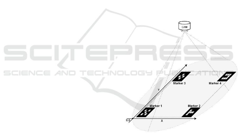
Subsequently, single markers must be positioned ho-

mogeneously in the environment within the camera’s

capture area. Precise measurements of the positioning

coordinates of each marker must be made, consider-

ing a Cartesian plane on the data collection surface.

This way, for each marker, we must have at least one

point p(x, y) with its coordinates, and more points can

be used. We use four points for each marker, where

each one is a vertex of the marker. Figure 1 shows a

representation of the camera positioning with markers

in the image capture area and the representation of the

X and Y axes of the Cartesian plane.

Figure 1: Environment illustration.

A new single marker must be positioned on top

of the robot. This marker will be the reference for

the robot’s positioning in the image captured by the

camera. Figure 2 shows the robot used in this work

with the marker positioned at its top.

4.1.1 Data Collect

After preparing the environment, the data of interest

can be collected. The collection is carried out syn-

chronously with the capture of each image from the

camera. Therefore, for each camera image saved, the

ICEIS 2024 - 26th International Conference on Enterprise Information Systems

120

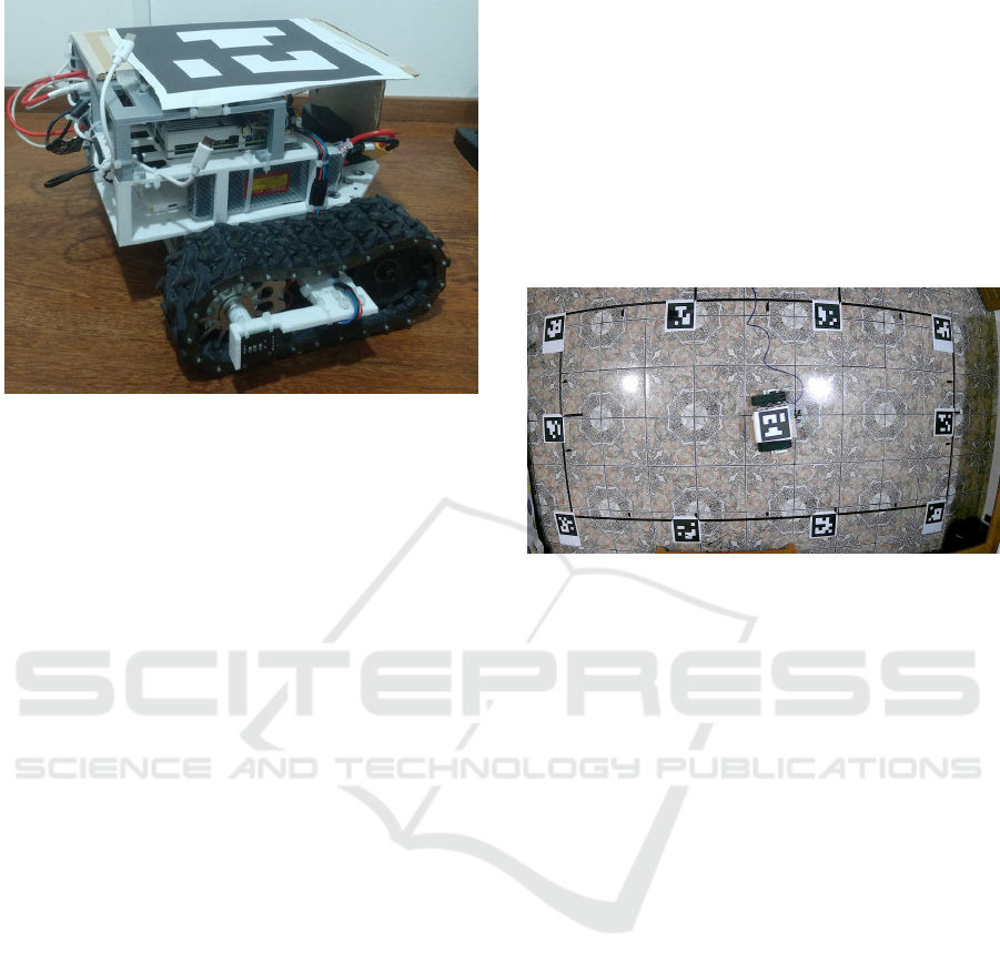
Figure 2: Marker on top of the robot.

time instant and measurements of each sensor in the

set of sensors used in the robot are also saved. In this

step, it is essential to make sure that image capture

and sensor data collection are synchronized.

Formally, we can represent data collection as fol-

lows. Consider each time instant t

in the collection

time interval, starting at t

and ending at t

. Data is

collected for each sensor s belonging to the set of sen-

sors S, and the image is saved at time t

. Synchronized

data collection can be represented by the Equation 4.

∀t

∈ [t

, t

] : ∀s ∈ S : Data(s, t

) ∪ Image(t

) (4)

In addition to taking care to synchronize data, two

rules must be considered during collection, which are:

1. Do not position the robot outside the camera cap-

ture area.

2. Do not obstruct the visibility of the marker posi-

tioned on top of the robot.

If one of the two previous rules were broken, there

would be an impact on the robot’s positioning ground

truth information. This breach will impact the detec-

tion of the robot’s marker, and when processing the

data, it will not be possible to detect the robot’s posi-

tion directly.

4.1.2 Data Processing

With the data in hand, they must be processed so that

the real positioning of the robot can be calculated at

each instant of time t

in which the data was captured.

A transformation is applied to the image collected by

the camera to calculate the real position of the robot

so that the image resulting from the transformation is

a representation of the Cartesian plane.

Considering that the image captured by the cam-

era is a representation of the Cartesian plane of the

surface of the data collection environment that has un-

dergone a T transformation, since the image is not an

orthogonal image due to the distortion caused by the

camera according to Figure 3. We can apply the in-

verse T

−1

transform to the captured image to obtain

each point in real space. In other words, we can ap-

ply T

−1

on the captured image in order to obtain the

correct representation of the Cartesian plane in a new

image.

Figure 3: Image originally captured.

The estimation of the T

−1

transformation is done

as follows. Let IP be the set of marker points detected

in the image captured by the camera, and RP be the set

of real positions of these points that were previously

measured during the environment setup stage. The in-

verse transformation T

−1

is estimated using the Thin

Plate Splines algorithm. The T

−1

transformation is

represented according to Equation 5.

−1

≈ T hinPlateSPLines(IP, RP) (5)

After applying the inverse transformation T

−1

the image, we can detect the marker attached to the

robot in the transformed image and consider a de-

tected position as the real position RPos of the robot

for the instant t

. In this way, after this detection, data

collection can be represented according to Equation

6, thus having data from the sensors and the robot’s

position at each instant of time t

. Figure 4 shows the

captured image after applying the inverse transforma-

tion.

∀t

∈ [t

, t

] : ∀s ∈ S : Data(s, t

) ∪ RPos(t

) (6)

If one of the two data collection rules is broken

or the robot mark is not detected in some frames, in-

terpolation can be applied to the positioning data to

ﬁll in the lost positions. One of the limitations of

this method is precisely the difﬁculty in detecting the

marker when the robot moves quickly. In Figure 5,

we show a summary of the data collection and pro-

A Computer Vision-Based Method for Collecting Ground Truth for Mobile Robot Odometry

121

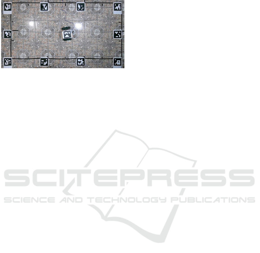
Figure 4: Image after inverse transformation has been ap-

plied.

cessing methodology. This method can be adjusted to

be used in extensive areas using a camera network.

5 EXPERIMENTS

In this section, we will present the experiments car-

ried out using the ground truth collection method pro-

posed in this work. Here, we show the robot used in

our data collection and how the data was collected.

Finally, we trained some DNNs on the data collected

using different sensors and compared the results.

5.1 Robot

Our crawler robot is based on ROBOCORE’s Raptor

platform (RoboCore, 2023). The robot has the fol-

lowing dimensions: 42 cm wide, 30 cm long, and 18

cm high. As actuators, the robot has 2 DC motors of

12 volts and 6500 rpm, each connected to a 16:1 re-

duction box, and the box shaft is connected directly

to the ring gear that moves the conveyor belt.

As a motor controller, we use a set of two hard-

ware, Raspberry Pi 4 model B (Raspberrypi, 2023)

and Brushed ESC 1060 (HOBBYWING, 2023),

which performs the driver function. The Raspberry

Pi 4 Model B has a 64-bit quad-core processor op-

erating at up to 1.5GHz and is sold in four different

RAM conﬁgurations: 1GB, 2GB, 4GB, and 8GB. In

this robot, we use the 4GB RAM model. Regarding

connectivity, it has a dual-band 2.4/5.0 GHz Wireless

adapter, Bluetooth 5.0/BLE, True Gigabit Ethernet,

USB 3.0, and power supply via USB-C. Additionally,

it supports two monitors at resolutions of up to 4K

at 60fps. Therefore, in this robot, our controller is a

composite hardware that we can divide into two parts,

with the Raspberry as the high-level controller and the

Brushed ESC 1060 as the low-level controller.

As an Edge AI device, we have an NVIDIA Jetson

Nano development kit (NVIDIA, 2023). Its CPU is

based on a 1.43 GHz 64-bit ARM Cortex-A57 Quad-

core CPU. It has a GPU with 128 NVIDIA CUDA

Cores, combined with 4 GB of LPDDR4x RAM. Its

connectivity is Gigabit Ethernet. It also has 4 USB 3.0

and HDMI video output. This platform does not have

a native wireless network, so we use a USB wireless

adapter for remote access.

We use two types of encoders for robot odome-

try and an IMU for sensing. From now on, we will

refer to the ﬁrst odometry as optical odometry as-

sembled by an encoder printed on a 3D printer and

a MOCH22A optical key module. The second odom-

etry is odometry carried out using a KY-040 rotary en-

coder. Figure 6 shows the positioning of the sensors

with the KY-040 coupled to the crown shaft and the

MOCH22A positioned to read the printed encoder.

The robot is also equipped with a Logitech C920

camera, 1080p and 30FPS. This camera was not used

in the experiments in which we only considered the

encoders and IMU proprioceptive sensors. In ﬁgure

7, we show the robot, highlighting its dimensions, the

positioning of its sensors, and the onboard computers.

The robot is controlled through a Python

client/server application developed with sockets, us-

ing the local Wi-Fi network infrastructure as a means

of communication.

5.2 Data Collection

Data was collected in an area measuring 1.5 m x 3

m. We used ArUco markers as markers both on the

ﬂoor and on the robot (Garrido-Jurado et al., 2014).

The camera used to collect data was connected to the

robot itself, more speciﬁcally to the NVIDIA Jetson

Nano, by using a 5-meter extension cable. This fea-

ture efﬁciently ensures the synchronous collection of

data from sensors and the camera that monitors the

environment. So, the collection followed Equation 6,

thus ensuring data sampling from all sensors for each

image synchronously collected by the camera.

We carried out 78 data collection sequences, 66

sequences lasting three minutes, nine sequences last-

ing 5 minutes, and three sequences lasting 10 min-

utes, totaling more than 4 hours and 30 minutes of

data collection, resulting in a total of 163920 sam-

ples. Data collection was carried out at an average

frequency of 9.5 Hz. During data collection, move-

ments were carried out in all directions, forwards and

backward, curves, and rotation movements around the

axis itself.

ICEIS 2024 - 26th International Conference on Enterprise Information Systems

122

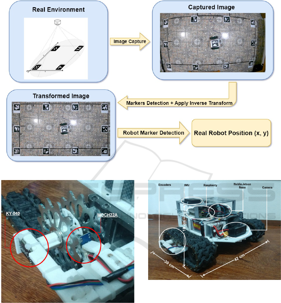
Figure 5: Complete methodology illustration.

Figure 6: Odometeres.

5.3 Odometry Comparison

The collected data was used to train neural networks

to perform comparisons. The comparison made here

assists in choosing which sensors we will use to im-

plement the robot’s odometry and validate the effec-

tiveness of the Ground Truth collection methodology.

We trained ﬁve neural networks, all with the same

architecture and varying the data used in training. The

architecture used was a fully connected neural net-

Figure 7: Robot.

work with 32, 32, 16, and 3 neurons in its ﬁrst, sec-

ond, third, and output layers, respectively. A dropout

layer with 10% probability between the third and out-

put layers was also used. Below, we show which sen-

sor data or combination was used to train each of the

5 DNNs.

1. Rotary Encoder (KY-040)

2. Optical Encoder (MOCH22A)

3. IMU

4. Rotary Encoder + IMU

5. Optical Encoder + IMU

A Computer Vision-Based Method for Collecting Ground Truth for Mobile Robot Odometry

123

In addition to the sensor data, each network also

used as an input parameter the time variation between

the current and last data sampling performed (∆t), the

last measured positioning variation (x

−1

− x

−2

, y

−1

−

−2

) and also the last orientation angle of the robot.

The networks used as expected output the variation in

positioning of the X and Y axes as well as the varia-

tion in the robot’s positioning angle. This way, odom-

etry is performed by adding the positioning variation

to the previous state. For encoders, the variation in

relation to the previous state is used at the input, and

for the IMU, raw data from the accelerometer and gy-

roscope were used.

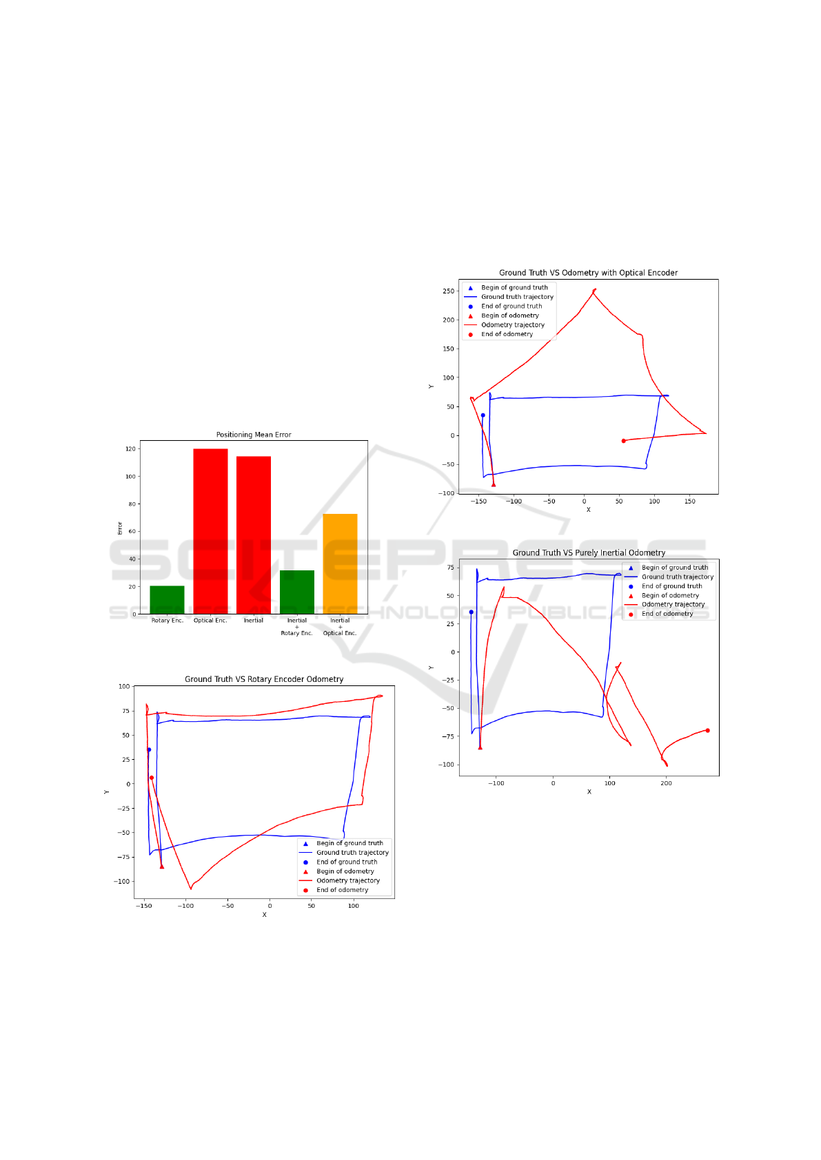
A path of 500 samples was chosen to compare the

odometry method, which was not used in the training

set. We compared the average positioning error on

this path as shown in Figure 8 and then plotted the

path described by each previously trained network.

Figure 8: Odometries positioning error.

Figure 9: Rotary encoder odometry trajectory.

Figure 8 shows that the smallest errors are when

using odometry with a rotary encoder and inertial

data combined with a rotary encoder. Optical encoder

odometry and purely inertial odometry presented the

highest error rates.

Figure 9 shows the odometry trajectory with ro-

tary encoder odometry compared to the ground truth

of the test path. Figure 10 shows the odometry trajec-

tory with optical encoder odometry compared to the

ground truth of the test path.

Figure 10: Optical encoder odometry trajectory.

Figure 11: Inertial odometry trajectory.

Figure 11 shows the purely inertial odometry tra-

jectory using only IMU data compared to the test

path’s ground truth. Figure 12 shows the odometry

trajectory with rotary encoder together with IMU data

compared to the ground truth of the test path.

Figure 13 shows the odometry trajectory with op-

tical encoder together with IMU data compared to the

ground truth of the test path.

When analyzing the graphs, we noticed that the

odometry methods that come closest to the path taken

ICEIS 2024 - 26th International Conference on Enterprise Information Systems

124

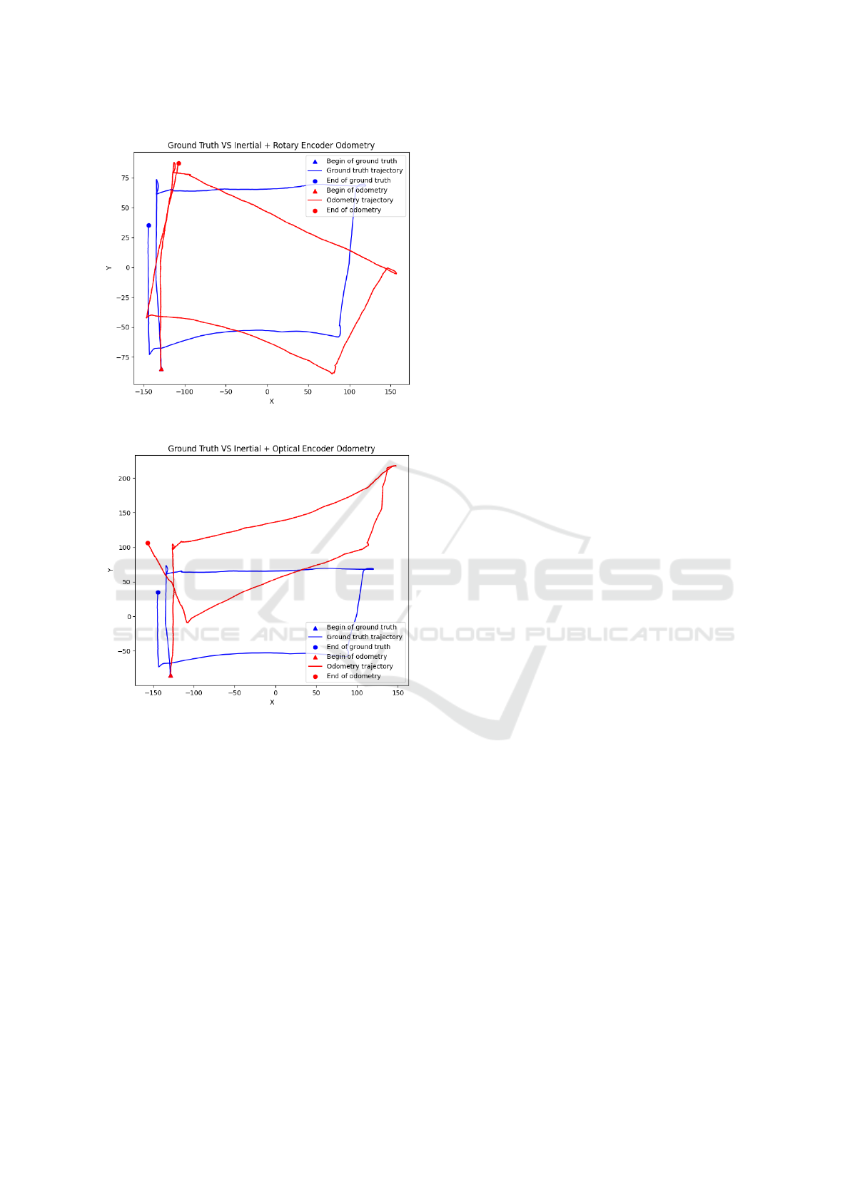
Figure 12: Inertial with rotary Encoder odometry.

Figure 13: Inertial with optical Encoder odometry.

in the ground truth are odometry with a rotary encoder

and odometry with a rotary encoder in conjunction

with IMU data, as well as in the comparison of the

average positioning error shown in Figure 8.

6 CONCLUSIONS

This paper presents a new methodology for collecting

ground truth for positioning robots in 2D space based

on computer vision. The proposed method requires

the preparation of the collection site, with the instal-

lation of a camera positioned higher than the environ-

ment to obtain broad images of the environment, in

addition to the use of markers both in the environment

and on the robot. The positioning of the markers must

be carried out following a Cartesian plane, and the po-

sitions must be carefully measured for later use in the

data processing stage. Data collection from sensors

and upper camera images must occur synchronously

to obtain consistent data.

After collection, the data goes through an essen-

tial processing process to map the position of the

markers identiﬁed in the camera image to an im-

age that represents their real positioning in the Carte-

sian plane of the collection environment. This trans-

formed image is used to detect the robot’s marker and

thus retrieve the actual position and orientation of the

robot. This method eliminates using simulated envi-

ronments, motion capture equipment, inertial visual

odometry (as in Google Tango), high-precision LI-

DARs, GPS or manual measurement during collec-

tion. In this way, it is more accessible and straightfor-

ward to implement, providing a more affordable ap-

proach. This contribution can boost the advancement

of research in mobile robotics, especially in the study

of land mobile robots.

In addition to the positioning ground generation

method proposal, a comparison between DNNs for

performing the odometry task was also presented. To

do this, we compare the use of data from different sen-

sors and their combination applied to a dense DNN.

Rotary encoders, optical encoders, and an IMU were

used during the collection. The results showed that

the best odometry methods were when the rotary en-

coder alone or in conjunction with IMU data was

used.

This work presents several possible sequences for

future work. Firstly, we will publish the database

generated during the collection process carried out in

the current study. We can then, for example, study

the possibility of adapting the methodology proposed

here for 3D environments, test the methodology in

more challenging locations, study odometry methods,

and compare them using our technique, among others.

ACKNOWLEDGEMENTS

The authors would like to thank MICHELIN Con-

nected Fleet, NVIDIA, UFOP, CAPES and CNPq for

supporting this work. This work was partially ﬁ-

nanced by Coordenac¸

ao de Aperfeic¸oamento de Pes-

soal de N

ıvel Superior (CAPES) - Finance Code

001, and by Conselho Nacional de Desenvolvimento

Cient

ıﬁco e Tecnol

ogico (CNPq) - Finance code

308219/2020-1.

A Computer Vision-Based Method for Collecting Ground Truth for Mobile Robot Odometry

125

REFERENCES

Alatise, M. B. and Hancke, G. P. (2020). A review on chal-

lenges of autonomous mobile robot and sensor fusion

methods. IEEE Access, 8:39830–39846.

Atik, M. E., Ozturk, O., Duran, Z., and Seker, D. Z. (2020).

An automatic image matching algorithm based on thin

plate splines. Earth Science Informatics, 13:869–882.

Ben-Ari, M., Mondada, F., Ben-Ari, M., and Mondada, F.

(2018). Robotic motion and odometry. Elements of

Robotics, pages 63–93.

Carlevaris-Bianco, N., Ushani, A. K., and Eustice, R. M.

(2016). University of michigan north campus long-

term vision and lidar dataset. The International Jour-

nal of Robotics Research, 35(9):1023–1035.

Ceriani, S., Fontana, G., Giusti, A., Marzorati, D., Mat-

teucci, M., Migliore, D., Rizzi, D., Sorrenti, D. G.,

and Taddei, P. (2009). Rawseeds ground truth collec-

tion systems for indoor self-localization and mapping.

Autonomous Robots, 27:353–371.

Chen, C., Zhao, P., Lu, C. X., Wang, W., Markham, A.,

and Trigoni, N. (2018). Oxiod: The dataset for deep

inertial odometry. arXiv preprint arXiv:1809.07491.

Cort

es, S., Solin, A., Rahtu, E., and Kannala, J. (2018). Ad-

vio: An authentic dataset for visual-inertial odometry.

In Proceedings of the European Conference on Com-

puter Vision (ECCV), pages 419–434.

Donato, G. and Belongie, S. (2002). Approximate thin plate

spline mappings. In Computer Vision—ECCV 2002:

7th European Conference on Computer Vision Copen-

hagen, Denmark, May 28–31, 2002 Proceedings, Part

III 7, pages 21–31. Springer.

Duchon, J. (1977). Splines minimizing rotation-invariant

semi-norms in sobolev spaces. In Constructive The-

ory of Functions of Several Variables: Proceedings of

a Conference Held at Oberwolfach April 25–May 1,

1976, pages 85–100. Springer.

Garrido-Jurado, S., Mu

noz-Salinas, R., Madrid-Cuevas,

F. J., and Mar

ın-Jim

enez, M. J. (2014). Auto-

matic generation and detection of highly reliable ﬁdu-

cial markers under occlusion. Pattern Recognition,

47(6):2280–2292.

Gurturk, M., Yuseﬁ, A., Aslan, M. F., Soycan, M., Durdu,

A., and Masiero, A. (2021). The ytu dataset and re-

current neural network based visual-inertial odometry.

Measurement, 184:109878.

HOBBYWING (2023). Esc1060. Available

in: https://www.hobbywing.com/en/products/

quicrun-wp-1060-brushed55.html. Accessed on

November 23, 2023.

Ishikawa, S. (1991). A method of indoor mobile robot

navigation by using fuzzy control. In Proceedings

IROS’91: IEEE/RSJ International Workshop on In-

telligent Robots and Systems’ 91, pages 1013–1018.

IEEE.

Khan, M. U., Zaidi, S. A. A., Ishtiaq, A., Bukhari, S. U. R.,

Samer, S., and Farman, A. (2021). A comparative

survey of lidar-slam and lidar based sensor technolo-

gies. In 2021 Mohammad Ali Jinnah University Inter-

national Conference on Computing (MAJICC), pages

1–8. IEEE.

Kirsanov, P., Gaskarov, A., Konokhov, F., Soﬁiuk, K.,

Vorontsova, A., Slinko, I., Zhukov, D., Bykov, S.,

Barinova, O., and Konushin, A. (2019). Discoman:

Dataset of indoor scenes for odometry, mapping and

navigation. In 2019 IEEE/RSJ International Confer-

ence on Intelligent Robots and Systems (IROS), pages

2470–2477. IEEE.

Mur-Artal, R., Montiel, J. M. M., and Tardos, J. D. (2015).

Orb-slam: a versatile and accurate monocular slam

system. IEEE transactions on robotics, 31(5):1147–

1163.

Niloy, M. A. K., Shama, A., Chakrabortty, R. K., Ryan,

M. J., Badal, F. R., Tasneem, Z., Ahamed, M. H.,

Moyeen, S. I., Das, S. K., Ali, M. F., Islam, M. R.,

and Saha, D. K. (2021). Critical design and control

issues of indoor autonomous mobile robots: A review.

IEEE Access, 9:35338–35370.

Nist

er, D., Naroditsky, O., and Bergen, J. (2004). Visual

odometry. In Proceedings of the 2004 IEEE Computer

Society Conference on Computer Vision and Pattern

Recognition, 2004. CVPR 2004., volume 1, pages I–I.

Ieee.

NVIDIA (2023). Nvidia jetson nano. Avail-

able in: https://developer.nvidia.com/embedded/learn/

get-started-jetson-nano-devkit. Accessed on Novem-

ber 23, 2023.

Perperoglou, A., Sauerbrei, W., Abrahamowicz, M., and

Schmid, M. (2019). A review of spline function pro-

cedures in r. BMC medical research methodology,

19(1):1–16.

Peynot, T., Scheding, S., and Terho, S. (2010). The maru-

lan data sets: Multi-sensor perception in a natural en-

vironment with challenging conditions. The Inter-

national Journal of Robotics Research, 29(13):1602–

1607.

Ramezani, M., Wang, Y., Camurri, M., Wisth, D., Mat-

tamala, M., and Fallon, M. (2020). The newer col-

lege dataset: Handheld lidar, inertial and vision with

ground truth. In 2020 IEEE/RSJ International Confer-

ence on Intelligent Robots and Systems (IROS), pages

4353–4360. IEEE.

Raspberrypi (2023). Raspberry pi 4 model b. Avail-

able in: https://www.raspberrypi.com/products/

raspberry-pi-4-model-b/. Accessed on November 23,

2023.

RoboCore (2023). Robocore. Available in: https://www.

robocore.net/roda-robocore/kit-raptor. Accessed on

November 23, 2023.

Rubio, F., Valero, F., and Llopis-Albert, C. (2019).

A review of mobile robots: Concepts, meth-

ods, theoretical framework, and applications. In-

ternational Journal of Advanced Robotic Systems,

16(2):1729881419839596.

Sokolov, S., Izmozherov, I., Blykhman, F., and Kutepov, S.

(2017). Thin plate splines method for 3d reconstruc-

tion of the left ventricle with use a limited number of

ultrasonic sections. DEStech Transactions on Engi-

neering and Technology Research, pages 258–262.

ICEIS 2024 - 26th International Conference on Enterprise Information Systems

126

Srinivas, P. and Kumar, A. (2017). Overview of architec-

ture for gps-ins integration. 2017 Recent Develop-

ments in Control, Automation & Power Engineering

(RDCAPE), pages 433–438.

Tzafestas, S. G. (2013). Introduction to mobile robot con-

trol. Elsevier.

Wang, H., Wang, C., Chen, C.-L., and Xie, L. (2021).

F-loam: Fast lidar odometry and mapping. In

2021 IEEE/RSJ International Conference on Intelli-

gent Robots and Systems (IROS), pages 4390–4396.

IEEE.

Wood, S. N. (2003). Thin plate regression splines. Jour-

nal of the Royal Statistical Society Series B: Statistical

Methodology, 65(1):95–114.

A Computer Vision-Based Method for Collecting Ground Truth for Mobile Robot Odometry

127