Explainable Machine Learning for Alarm Prediction

Kalleb M. M. Abreu

1 a

, Julio C. S. Reis

1 b

, Andr

e Gustavo dos Santos

1 c

and Giorgio Zucchi

2 d

Department of Informatics, Universidade Federal de Vic¸osa, Minas Gerais, Brazil

R&D Department, Coopservice s.c.p.a, Reggio Emilia, Italy

Keywords:

Alarms, Machine Learning, Clustering, Classiﬁcation, Explainable Model.

Abstract:

This paper evaluates machine learning models for the prediction of alarms using geographical clustering, ex-

ploring data from an Italian company. The models encompass a spectrum of algorithms, including Naive

Bayes (NB), XGBoost (XGB), and Multilayer Perceptron (MLP), coupled with encoding techniques, and

clustering methodologies, namely COOP (Coopservice) and KPP (K-Means++). The XGB models emerge as

the most effective, yielding the highest AP (Average Precision) values across models based on MLP and NB.

Hyperparameter tuning for XGB models reveals default values perform well. Our model explainability analy-

ses reveal the signiﬁcant impact of geographical location (cluster) and the time interval when the predictions

are made. Challenges arise in handling dataset imbalances, impacting minority alarm class predictions. the

insights gained from this study lay the groundwork for future investigations in the ﬁeld of geographical alarm

prediction. The identiﬁed challenges, such as imbalanced datasets, offer opportunities for reﬁning methodolo-

gies. As we move forward, a deeper exploration of one-class algorithms holds promise for addressing these

challenges and enhancing the robustness of predictive models in similar contexts.

1 INTRODUCTION

Alarm systems are crucial for safeguarding individu-

als, properties, and assets, acting as deterrents to po-

tential criminals and enabling prompt responses from

security teams or police upon activation (Rutgers Uni-

versity, 2009). Predicting alarms aids patrol manage-

ment, reducing intervention time by assigning guards

to high-risk areas. Machine learning models have

been applied in various scenarios, enhancing accuracy

and efﬁciency in alarm prediction (Au-Yeung et al.,

2019; Meng and Kwok, 2012; Quinn, 2020; Zhuang

et al., 2020). These efforts optimize resource alloca-

tion and improve security measures in network sys-

tems (Lateano et al., 2023; Zhang and Wang, 2019)

and industries (Zhu et al., 2016).

While previous studies focus on alarm predic-

tion, they often overlook geographic locations and

lack model explainability. This work addresses these

gaps by emphasizing the geographic aspect of alarms

and prioritizing model explainability. The study

uses real data from Coopservice, an Italian service

https://orcid.org/0000-0001-8905-2402

https://orcid.org/0000-0003-0563-0434

https://orcid.org/0000-0002-5743-3523

https://orcid.org/0000-0002-5459-7290

provider offering logistics, transportation, cleaning,

maintenance, and security services, particularly car

patrolling in various provinces. Coopservice utilizes a

cluster system to optimize its routes and enhance pa-

trol efﬁciency (Zucchi et al., 2022). When alarms oc-

cur, patrols are dispatched, impacting deﬁned routes.

To minimize this impact, alarm prediction within each

cluster is crucial for considering the probability of

alarm incidents when generating routes. Leverag-

ing robust machine learning algorithms, this work ex-

plores the use of such tools for alarm prediction.

Thus, the main objective of this paper is to con-

duct an analysis using real data to achieve effective

alarm prediction. The study aims to explore Ma-

chine Learning algorithms that can accurately pre-

dict alarms within a one-hour time interval to assist

companies in their efforts to manage and respond to

alarms effectively. Furthermore, the research com-

pares models based on patrols, where each patrol cor-

responds to a cluster, deﬁned in two ways: (i) the cur-

rent clusters deﬁned by the company and (ii) those

determined through the k-means clustering algorithm.

To facilitate the end user’s interaction with the pro-

posed approach, we explore aspects of explainability.

This allows for a clearer understanding of the model’s

decision-making process and enhances the system’s

690

Abreu, K., Reis, J., Santos, A. and Zucchi, G.

Explainable Machine Learning for Alarm Prediction.

DOI: 10.5220/0012625000003690

Paper published under CC license (CC BY-NC-ND 4.0)

In Proceedings of the 26th International Conference on Enterprise Information Systems (ICEIS 2024) - Volume 1, pages 690-697

ISBN: 978-989-758-692-7; ISSN: 2184-4992

usability. We expect that the strategies presented in

this work will provide valuable assistance to compa-

nies in optimizing their patrol services.

In addressing the aforementioned objectives, it is

essential to highlight that the existing literature lacks

comprehensive coverage of scenarios wherein deter-

mining not only the occurrence of alarms but also

their geographical location is crucial. This gap be-

comes particularly signiﬁcant in our context, where

understanding the impact of alarms on predeﬁned car

patrolling routes is paramount. Notably, the literature

also falls short in exploring the explainability of mod-

els within this speciﬁc domain. In contrast to prior

efforts, this study seeks to identify machine learning

algorithms capable of predicting alarms within clus-

ters, considering their geographic aspects.

The rest of the paper is organized as follows. In

Section 2, we present relevant related work. Section

3 provides a formal problem deﬁnition and introduces

the dataset used in the study. In Section 4, we present

the proposed models, tuning of hyperparameters, and

analysis of the best-performing models. Last, Section

5 presents our conclusions.

2 RELATED WORK

Several stakeholders are interested in alarm-related

works (Au-Yeung et al., 2019; Lateano et al., 2023;

Zhang and Wang, 2019) to minimize the time between

the alarm and remedial action or implement preven-

tive measures. We can group the machine learning re-

search lines applied to alarms into two sets: (i) ﬁlter-

ing and (ii) prediction. Within the (i) ﬁltering research

works, we observe studies developed to identify false

alarms. The work of (Meng and Kwok, 2012), for

instance, highlight the issue of the high number of

false alarms generated in intrusion detection systems

(IDSs) and ﬁnds relevant results by applying machine

learning models. On the other hand, Au-Yeung et al.

(2019) deal with alert alarms in intensive care units

(ICUs) responsible for reporting changes in patient’s

psychological signals. In many situations, interven-

tions are unnecessary, and the alarms become a bur-

den. Additionally, excessive alarms in these environ-

ments can cause noise disturbances.

The efforts that follow the (ii) prediction line

mainly serve the industry and network systems. In

the industrial scenario, we have (Zhu et al., 2016) who

apply a probabilistic model to calculate the probabil-

ity of critical alarm occurrence. Quinn (2020) found

excellent results by applying artiﬁcial neural networks

to predict pressure alarms in natural gas pipelines. On

the other hand, Pezze et al. (2022) develop a Deep

Learning-based approach for predicting alarms in in-

dustrial equipment, representing a low-cost alterna-

tive to sensor-based preventive maintenance strate-

gies. In the context of networks, Zhang and Wang

(2019) propose an alarm analysis scheme for predict-

ing faults in optical transport networks using support

vector machines (SVM) and long short-term mem-

ory (LSTM). Zhuang et al. (2020) address the same

problem, who use a self-optimizing data augmenta-

tion method based on generative adversarial networks

(GANs); the results in commercial tests achieve high

accuracy. Finally, Lateano et al. (2023) address the

prediction of failures in networks through the analy-

sis of real alarm data from microwave network equip-

ment.

However, the works in both groups (i) and (ii) do

not address scenarios where it is important to deter-

mine not only the occurrence of the alarm but also its

geographic location. Unlike previous studies, these

scenarios are extremely relevant to our problem, given

that it is crucial in determining the impact of alarms

on the routes practiced in car patrolling. For example,

a car moves according to the deﬁned route to patrol

the area, but an alarm is triggered during the displace-

ment. Since alarms represent a possibility of security

vulnerability, the patrol must respond to the call, de-

viating from the planned route. The impact of these

trajectory alterations over the year can mean a consid-

erable increase in the operation cost. Moreover, to the

best of our knowledge, there is a lack of research ex-

ploring the explainability of models within this con-

text. Thus, different from previous efforts, this work

seeks to determine machine learning algorithms that

can assist in predicting these alarms within clusters

while investigating their explainability, which would

be a signiﬁcant contribution to the ﬁeld of alarm pre-

diction.

3 PROBLEM DEFINITION AND

DATASET

This section introduces the alarm detection problem

using Coopservice’s patrol data. In Section 3.1, we

formally deﬁne the problem as developing a model

for detecting alarms and assigning likelihood scores

within speciﬁc clusters and time intervals. Section 3.2

presents the dataset, focusing on the studied province

and key alarm-related information. The distribution

of alarms is analyzed based on variations in month

and hour. Section 3.3 outlines the process of cluster-

ing alarms, using the K-Means++ algorithm (Arthur

and Vassilvitskii, 2007) for theoretical comparison.

Last, we discuss creating negative instances, gener-

Explainable Machine Learning for Alarm Prediction

691

ating features based on date and time, and describe

the encoding method for each feature, providing a

comprehensive overview for subsequent analysis and

model development.

3.1 Deﬁnition

Formally, we can deﬁne the problem of alarm detec-

tion considering geographical location as follows:

Deﬁnition 3.1. (Alarms Detection) Given a clus-

ter c ∈ C, and a time interval t ∈ T, a model for alarm

detection assigns a score S(c, t) ∈ [0, 1] indicating the

extent to which the pair c,t is believed to have an

alarm. A threshold τ can be deﬁned such that the pre-

diction function F : C, T → {alarm, not alarm} is:

F(c,t) =

(

alarm, if S(c, t) > τ

not alarm, otherwise.

Our cluster deﬁnition assigns a speciﬁc geo-

graphic region for a car patrol to operate.

3.2 Overview of Dataset

The car patrol dataset from Coopservice in Italy pro-

vides rich information, featuring data from 150 pa-

trols across 30+ cities. With over 150,000 alarms

recorded between January 1, 2020, and November 6,

2022, the dataset includes essential ﬁelds like date,

geographic location (i.e., latitude and longitude), ac-

tivity type, and the associated car patrol. This dataset

offers a detailed and comprehensive perspective on

Coopservice’s car patrol activities.

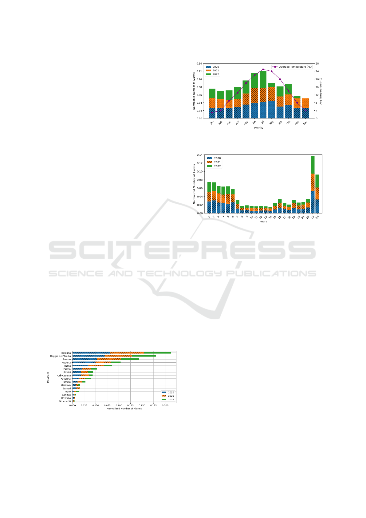
This study concentrates on analyzing alarms in

Reggio Emilia, selected due to its notable alarm activ-

ity, as illustrated in Figure 1, and its strategic signiﬁ-

cance to the company. In Figure 2, we observe the dis-

tribution of normalized alarm numbers per month and

hour. Figure 2a portrays a consistent pattern in alarm

distribution over the years, except for August 2022.

Figure 1: Number of alarms by province. The graphs show

the number of alarms per hour and per month, with the y-

axis values normalized using the min-max normalization

technique. This process ensures that the values are scaled

between 0 and 1.

(a) Number of alarms and max temperature by months in Reg-

gio Emilia.

(b) Number of alarms by hours.

Figure 2: The graphs show the number of alarms per month

and hour, with the y-axis values normalized using the min-

max normalization technique. This process ensures that the

values are scaled between 0 and 1.

Data for November 2022 is incomplete, and Decem-

ber 2022 has no available data. The occurrences of

alarms tend to increase from April to October, align-

ing with rising temperatures and a decline in outdoor

activities during colder months. Warmer seasons, in-

cluding Italian summer holidays, witness heightened

mobility, especially towards coastal areas. The cir-

culation of people appears to be correlated with the

incidence of alarms.

Figure 2b shows higher alarm occurrences during

the night, peaking at 23 hours. Data collection during

the COVID-19 pandemic impacted alarm distribution,

with protective measures inﬂuencing the numbers.

3.3 Dataset Preprocessing

To prepare our dataset for predictions, we conduct es-

sential data cleaning steps, addressing missing values

and duplicates. Further details on additional steps are

provided in the following sections: Dataset Clustering

(Section 3.3.1), Non-alarm Instances (Section 3.3.2),

Feature Deﬁnition and Encoding (Section 3.3.3) and

Data Processing Pipeline (Section 3.3.4).

ICEIS 2024 - 26th International Conference on Enterprise Information Systems

692

3.3.1 Dataset Clustering

According to Deﬁnition 3.1, the problem involves

classifying events into alarms or non-alarms within a

time interval in a cluster. Understanding information

about alarm clusters is crucial for optimizing patrol

routes. Currently, Coopservice’s alarm response pro-

cess considers the patrol closest to the event, irrespec-

tive of the predeﬁned cluster for that patrol.

In our dataset, we have cluster information for pa-

trols during non-alarm activities. Using the convex

hull algorithm, we deﬁne the convex region represent-

ing each cluster. The convex hull is the smallest con-

vex polygon encompassing all given points, visual-

ized as the outer boundary.

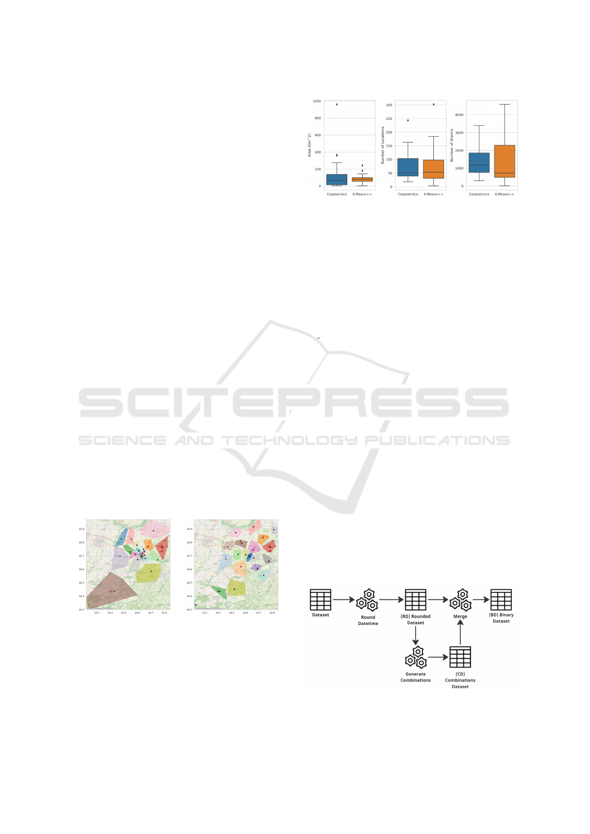
Coopservice operates with 20 patrols in Reggio

Emilia province, each represented by a distinct con-

vex region, as shown in Figure 3a. These regions

serve as clusters for alarm response. Cluster sizes

and the number of locations vary signiﬁcantly, based

on Coopservice’s established practices. Some patrols

may be overloaded, covering numerous locations or

long distances, while others may be less occupied.

For comparison, we employ the K-Means++ algo-

rithm, selecting k = 20 to match Coopservice’s clus-

ters. Distances between alarms and centroids were

computed based on latitude and longitude. The re-

sults are depicted in Figure 3b.

The convex regions from both methods signiﬁ-

cantly differ in area, location count, and alarm dis-

tribution, as seen in Figure 4. K-Means++ yields

smaller patrol coverage areas, potentially reducing

travel time. However, it exhibits extremes in loca-

tion and alarm distribution, with some clusters having

high activity and others being more idle compared to

Coopservice’s established distribution.

(a) Convex regions ob-

tained through Coopservice

patrols.

(b) Convex regions ob-

tained through K-Means++.

Figure 3: Convex regions of clusters formed through geo-

graphical locations. The centroid of the points in each con-

vex region is represented by a black triangle.

Figure 4: Boxplot comparing covered area, number of lo-

cations, and alarm distribution of convex regions generated

by Coopservice and K-Means++ methods.

3.3.2 Non-Alarm Instances

In the preceding section, we outlined how we de-

ﬁned clusters, resulting in two datasets: one based

on Coopservice’s practices (COOP) and another using

K-Means++ with k equal to 20 (KPP). Both datasets

have two columns: datetime (alarm occurrence times-

tamp in yyyy-MM-dd hh-mm-ss format) and clus-

ter

code. Our prediction function, per Deﬁnition 3.1,

classiﬁes outcomes as alarm or not alarm based on a

deﬁned threshold. However, our dataset only contains

alarm occurrences, lacking negative instances. To ad-

dress this, we introduce negative occurrences through

the three-step process detailed below.

Figure 5 illustrates the steps for generating our

binary dataset (BD) with positive and negative oc-

currences. Focusing on the one-hour interval, our

ﬁrst step involves rounding datetime by hour, creat-

ing the rounded dataset (RD). The second step gener-

ates hourly datetime entries for each cluster on the

ﬁrst and last day through RD, forming the combi-

nations dataset (CD). For instance, a 10-day interval

with ﬁve clusters results in 1200 instances (10 days

x 24 hours x 5 clusters). Finally, we join RD and

CD, retaining all CD entries. We label entries in both

datasets as alarm and those only in CD as no alarm,

as RD only contains alarm occurrences. The result-

ing binary dataset (BD) has two classes: alarm and no

alarm, with 475,152 non-alarm instances, following

the same steps for COOP and KPP.

Figure 5: Steps to generate the binary dataset BD that in-

cludes both classes: alarm and no alarm.

Explainable Machine Learning for Alarm Prediction

693

Table 1: Properties of the features for the datasets.

Feature Type Encoding

year Discrete Label/Ordinal

month Discrete Label/Ordinal

day Discrete Label/Ordinal

hour Discrete Label/Ordinal

shift Ordinal Label/Ordinal

day of week Ordinal Label/Ordinal

cluster code Nominal

One-Hot

Label/Ordinal

3.3.3 Feature Deﬁnition and Encoding

The ﬁnal data processing step involves feature deﬁni-

tion and encoding. Our datasets contain two columns:

datetime and cluster code. Using the datetime col-

umn, we generate temporal features: year, month,

day, hour, shift, and day

of week. These features help

us understand the relevance of individual time charac-

teristics for our model or their combined evaluation.

Table 1 displays the model features, data types, and

encoding methods.

3.3.4 Data Processing Pipeline

We generate four datasets using two clustering mod-

els (COOP and KPP) and two encoding methods

for cluster code: Label/Ordinal Encoding (LOE) and

Label/Ordinal/One-hot Encoding (L2OE). Figure 6

illustrates the sequential steps in our data process-

ing pipeline. Initially, we extract patrol data from

the Coopservice database and use the ArcGIS API

to obtain address information, transforming latitude

and longitude into city, province, and other details.

This forms the Base Dataset. Applying Coopser-

vice’s clustering methods, K-Means++, and a non-

alarm creation function, we create the COOP and KPP

datasets. Through encoding techniques, we produce

the ﬁnal datasets for model training.

The datasets comprise 499,680 instances, cover-

ing alarm occurrences and non-occurrences. LOE

datasets have 7 features, while L2OE datasets boast

26 features due to One-Hot Encoding transforming

Figure 6: Illustration of the data processing pipeline.

https://developers.arcgis.com/python/

the cluster code feature into 20 features, each cor-

responding to a distinct cluster. The datasets exhibit

an imbalance, with only 5% of instances representing

alarm occurrences, yielding a ratio of 1 occurrence for

every 19 non-occurrences. Notably, the alarm occur-

rences in this dataset do not represent the total number

attended by Coopservice. As a cluster comprises mul-

tiple locations, an alarm in any location within a spe-

ciﬁc cluster deﬁnes an instance with an alarm in our

problem. Thus, a cluster can have multiple alarms in

a time interval without affecting our model, consider-

ing an alarm occurrence if the count is greater than 0;

otherwise, it is a non-occurrence.

4 MODELING AND ANALYSIS

This section explores model selection, evaluation, and

reﬁnement for three machine learning models: Naive

Bayes (NB), eXtreme Gradient Boosting (XGB), and

Multilayer Perceptron Classiﬁer (MLP). The focus is

on the efﬁciency of these models in predicting alarm

occurrences using two clustering methods: ORG-

2022 (COOP) and K-Means++ (KPP). Thorough as-

sessments, primarily using the AP metric.

The exploration includes hyperparameter opti-

mization, particularly for the XGB algorithm, aimed

at improving model performance. Advanced interpre-

tative techniques like the SHAP framework are also

employed to understand feature importance and the

inﬂuence of various factors on alarm classiﬁcation.

Subsequent sections detail model selection in Section

4.1, hyperparameter optimization in Section 4.2, and

the analysis of the best models in Section 4.3.

4.1 Model Selection

The dataset covers 1041 days from January 1, 2020, to

November 6, 2022. Models are trained on 720 days,

representing 69.09% of the total, with a temporal split

ensuring that test data occurs entirely after the train-

ing set, minimizing bias. The remaining portion is

dedicated solely to model evaluation.

Three machine learning approaches are selected

for the study: Naive Bayes (NB) (Hand and Yu,

2001), eXtreme Gradient Boosting (XGB) (Chen and

Guestrin, 2016), and Multilayer Perceptron Classiﬁer

(MLP) (Murtagh, 1991). These models represent dif-

ferent machine learning families: NB is probabilistic,

XGB is an ensemble, and MLP belongs to artiﬁcial

neural networks. Training is conducted on Google

Colab using Python 3, importing NB and MLP from

Scikit-Learn and XGB from the xgboost library.

Default conﬁgurations are used from the libraries,

ICEIS 2024 - 26th International Conference on Enterprise Information Systems

694

along with identical training and test sets for a fair

comparison. Evaluation utilizes the area under the PR

curve (AP) metric, suitable for imbalanced datasets.

Our tests showed that the best model was generated

through XGB, in all scenarios (LOE, L2OE, KPP,

and COOP). Therefore, we decided to proceed with

hyperparameter optimization for XGB in order to

achieve better performance.

4.2 Hyperparameter Optimization

Our hyperparameter tuning process involves optimiz-

ing the settings of the XGB algorithm to enhance

its performance in predicting alarm occurrences. To

achieve this, we utilize a 10-fold cross-validation ap-

proach, splitting the training data into folds with dis-

tinct distributions for training, validation, and testing.

Each fold represents a 72-day interval, with a training

period of 36 days, followed by 18 days for validation

and another 18 days for testing.

The primary goal of this approach is to ensure that

the selected hyperparameters are not overly depen-

dent on speciﬁc characteristics of the training data.

By using small samples in each fold, we aim to create

a model that generalizes well to new information and

avoids overﬁtting issues. This separation into train-

ing, validation, and testing sets aids in the robust eval-

uation of the model’s performance.

In our hyperparameter tuning process, we allo-

cate the remaining 321 days for the ﬁnal evaluation of

model AP scores. Due to the time series nature of the

problem, we adopt isolated block-wise splits, train-

ing models on one portion of the dataset, and evaluat-

ing them on subsequent chronological sections. This

practice mimics real-world scenarios where only his-

torical data is available for prediction.

Among the considered hyperparameters, we

focus on key parameters widely applicable in

XGB and other tree-based models (Developers,

2023): max depth, learning rate, n estimators,

early stopping rounds.

Throughout the 10-fold cross-validation, the con-

ﬁguration with the best average AP across folds is

considered the optimal set of hyperparameters. Selec-

tion is based on information from the XGB documen-

tation (Developers, 2023) and the Analytics Vidhya

blog’s guide on XGB parameter tuning (Jain, 2016),

recommended by Awesome XGB

(DMLC, 2023).

Table 2 shows a summary of the AP obtained

from the models with default hyperparameters and

the tuned ones. The table indicates that the models

Awesome XGB is mentioned in the documen-

tation as a source of resources on XGB, available at

https://xgboost.readthedocs.io/en/stable/tutorials/index.html.

Table 2: AP comparison for XGB models trained with dis-

tinct clustering and encoding methods.

Models Default Tuned Improvement

xgb coop loe 0.149 0.154 0.5%

xgb coop l2oe 0.148 0.155 0.7%

xgb kpp loe 0.190 0.197 0.7%

xgb kpp l2oe 0.190 0.197 0.7%

did not show signiﬁcant performance improvements,

with only a 0.7% increase in AP for the KPP models

in the best case scenario. However, it is important to

note that the choice of clustering method has a more

substantial impact on the models, resulting in an ap-

proximately 4% increase in AP for the KPP models

compared to the COOP models.

For XGB models, exclusive use of Label/Ordinal

Encoding (LOE) is favored over One-Hot Encod-

ing due to comparable performance and simplicity.

LOE’s fewer features enhance model evaluation and

enable seamless applicability to datasets with con-

sistent feature numbers, fostering adaptability across

provinces with varying patrol counts. This choice

aligns with a straightforward and efﬁcient approach to

data analysis, opening possibilities for transfer learn-

ing applications in diverse scenarios.

4.3 Analysis of Optimal Models

When dealing with complex machine learning mod-

els, it is important to be able to interpret their predic-

tions. However, achieving both accuracy and inter-

pretability can be challenging. A framework called

SHapley Additive exPlanations (SHAP) was devel-

oped by Lundberg and Lee (2017) to address this

problem. SHAP assigns importance values to fea-

tures for speciﬁc predictions, offering a uniﬁed and

theoretically supported approach. Widely used for

enhancing model interpretability, SHAP is chosen in

this work, following precedents in studies like (Li,

2022), (Ekanayake et al., 2022), and (Mangalathu

et al., 2020).

For the xgb coop loe model, Figure 7 illus-

trates SHAP information. The feature ranking

highlights the crucial impact of hour, cluster code,

and day of week, with signiﬁcantly higher absolute

SHAP values compared to other features. The dis-

tribution of feature values against SHAP values, re-

veals how different features impact the classiﬁcation

of alarm occurrences or non-occurrences. The distri-

bution, aligned with SHAP values, highlights that ex-

treme hours (both low and high) and weekends pos-

itively inﬂuence alarm occurrences, often associated

with minimal pedestrian trafﬁc, particularly during

sleeping hours.

Explainable Machine Learning for Alarm Prediction

695

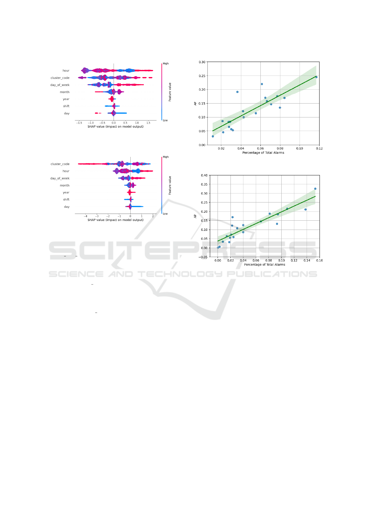
Figure 7: Feature importance and distribution analysis us-

ing SHAP scores for the COOP model.

Figure 8: Feature importance and distribution analysis us-

ing SHAP scores for the KPP model.

In Figure 8, a parallel analysis is conducted for

the xgb kpp loe model, mirroring the approach taken

with the previous model. The ﬁndings reveal a

model emphasis on times with low pedestrian traf-

ﬁc and weekends for KPP. A noteworthy difference

surfaces as cluster

code emerges as the most crucial

feature, underscoring its signiﬁcance in enhancing the

model’s performance. Interestingly, the contribution

of each feature to the models shows closely aligned

values, with cluster code standing out with notably

higher importance.

Analyzing the correlation between the model’s AP

for each cluster and the percentage of alarms within

clusters in Figure 9 reveals intriguing relationships.

For COOP in Figure 9a, and KPP in Figure 9b there’s

a positive correlation of 0.830 and 0.900, respectivaq-

mente. Clusters with more alarms are more readily

assessed by the XGB model.

These observations underscore the varied impli-

cations of alarm distribution within clusters on model

efﬁcacy. Employing k-means for distribution yielded

clusters with higher alarm density compared to the

strategy employed by Coopservice. Consequently,

clusters exhibiting higher alarm density demonstrate

superior performance in alarm prediction. This ﬁnd-

ing sheds light on the crucial role of data distribution

strategies in optimizing predictive model outcomes.

As clusters play a crucial role in alarm predic-

(a) AP and alarm percentage for COOP clusters.

(b) AP and alarm percentage for KPP clusters.

Figure 9: Comparative analysis of AP-alarm percentage

correlations for COOP and KPP clusters.

tions, enhancing collaboration between the route op-

timizer and the alarm predictor is relevant. Assign-

ing an AP score to each cluster and time of day is a

promising approach. The optimizer can then priori-

tize alarm predictions for clusters and time slots with

higher scores, reducing signiﬁcance for those with

lower accuracy.

This strategy optimizes resource allocation, en-

hancing the efﬁciency of the alarm response sys-

tem. Patrol teams are dispatched more reliably, reduc-

ing unnecessary deployments to regions with lower

prediction accuracy. Incorporating AP scores into

decision-making ﬁne-tunes the system to each clus-

ter’s characteristics and variations in alarm occur-

rence patterns throughout the day.

ICEIS 2024 - 26th International Conference on Enterprise Information Systems

696

5 CONCLUSIONS

Our paper evaluated machine learning models across

three algorithms, two encoding methods, and two

clustering techniques for alarm prediction using

data from an Italian company. XGB, particularly

with K-Means++ clustering, showed the highest

performance. Despite hyperparameter tuning,

improvements were marginal. SHAP analysis em-

phasized key features like cluster identiﬁcation and

alarm time. However, further study is needed as our

best scenarios fell below 0.5 AP. As future work,

we intend to explore techniques for dealing with

highly unbalanced datasets or one-class classiﬁcation

algorithms.

ACKNOWLEDGEMENTS

K. Abreu, J. Reis, and A. Santos are grateful to

CAPES and FAPEMIG for funding different parts of

this work.

REFERENCES

Arthur, D. and Vassilvitskii, S. (2007). K-means++: The

advantages of careful seeding. In Proceedings of the

Eighteenth Annual ACM-SIAM Symposium on Dis-

crete Algorithms, SODA ’07, page 1027–1035, USA.

Society for Industrial and Applied Mathematics.

Au-Yeung, W.-T. M., Sahani, A. K., Isselbacher, E. M., and

Armoundas, A. A. (2019). Reduction of false alarms

in the intensive care unit using an optimized ma-

chine learning based approach. npj Digital Medicine,

2(1):86.

Chen, T. and Guestrin, C. (2016). XGBoost. In Proceedings

of the 22nd ACM SIGKDD International Conference

on Knowledge Discovery and Data Mining. ACM.

Developers, X. (2023). Xgboost documentation.

https://xgboost.readthedocs.io/en/stable/index.html.

Accessed on: November 30, 2023.

DMLC (2023). Xgboost: Scalable and ﬂexible gradient

boosting. https://github.com/dmlc/xgboost.

Ekanayake, I., Meddage, D., and Rathnayake, U. (2022). A

novel approach to explain the black-box nature of ma-

chine learning in compressive strength predictions of

concrete using shapley additive explanations (shap).

Case Studies in Construction Materials, 16:e01059.

Hand, D. J. and Yu, K. (2001). Idiot’s bayes: Not so stupid

after all? International Statistical Review / Revue In-

ternationale de Statistique, 69(3):385–398.

Jain, A. (2016). Mastering xgboost parameter tuning: A

complete guide with python codes. Accessed on 2023-

11-30.

Lateano, F., Ayoub, O., Musumeci, F., and Tornatore, M.

(2023). Machine-learning-assisted failure prediction

in microwave networks based on equipment alarms.

In 2023 19th International Conference on the Design

of Reliable Communication Networks (DRCN), pages

1–7.

Li, Z. (2022). Extracting spatial effects from machine learn-

ing model using local interpretation method: An ex-

ample of shap and xgboost. Computers, Environment

and Urban Systems, 96:101845.

Lundberg, S. M. and Lee, S.-I. (2017). A uniﬁed approach

to interpreting model predictions. In Proceedings of

the 31st International Conference on Neural Informa-

tion Processing Systems, NIPS’17, page 4768–4777,

Red Hook, NY, USA. Curran Associates Inc.

Mangalathu, S., Hwang, S.-H., and Jeon, J.-S. (2020).

Failure mode and effects analysis of rc members

based on machine-learning-based shapley additive ex-

planations (shap) approach. Engineering Structures,

219:110927.

Meng, Y. and Kwok, L.-f. (2012). Adaptive false alarm ﬁl-

ter using machine learning in intrusion detection. In

Wang, Y. and Li, T., editors, Practical Applications

of Intelligent Systems, pages 573–584, Berlin, Heidel-

berg. Springer Berlin Heidelberg.

Murtagh, F. (1991). Multilayer perceptrons for classiﬁca-

tion and regression. Neurocomputing, 2(5):183–197.

Pezze, D. D., Masiero, C., Tosato, D., Beghi, A., and Susto,

G. A. (2022). Formula: A deep learning approach for

rare alarms predictions in industrial equipment. IEEE

Transactions on Automation Science and Engineer-

ing, 19(3):1491–1502.

Quinn, C. (2020). Alarm forecasting in natural gas

pipelines. Master’s thesis, Milwaukee, Wisconsin.

Rutgers University (2009). Rutgers study ﬁnds

alarm systems are valuable crime-ﬁghting tool.

https://www.rutgers.edu/news/rutgers-study-ﬁnds-

alarm-systems-are-valuable-crime-ﬁghting-tool.

Accessed on May 15, 2023.

Zhang, M. and Wang, D. (2019). Machine learning based

alarm analysis and failure forecast in optical net-

works. In 2019 24th OptoElectronics and Commu-

nications Conference (OECC) and 2019 International

Conference on Photonics in Switching and Computing

(PSC), pages 1–3.

Zhu, J., Wang, C., Li, C., Gao, X., and Zhao, J. (2016).

Dynamic alarm prediction for critical alarms using a

probabilistic model. Chinese Journal of Chemical En-

gineering, 24(7):881–885.

Zhuang, H., Zhao, Y., Yu, X., Li, Y., Wang, Y., and Zhang,

J. (2020). Machine-learning-based alarm prediction

with gans-based self-optimizing data augmentation in

large-scale optical transport networks. In 2020 Inter-

national Conference on Computing, Networking and

Communications (ICNC), pages 294–298.

Zucchi, G., Corr

ea, V. H., Santos, A. G., Iori, M., and Yag-

iura, M. (2022). A metaheuristic algorithm for a multi-

period orienteering problem arising in a car patrolling

application. In INOC, pages 99–104.

Explainable Machine Learning for Alarm Prediction

697