Optimizing Planning Strategies: A Machine Learning Forecasting

Model for Energy Aggregators and Hydropower Producers

Sarah Di Grande

, Mariaelena Berlotti

, Salvatore Cavalieri

and Roberto Gueli

Department of Electrical Electronic and Computer Engineering, University of Catania, Viale A.Doria n.6, Catania, Italy

EHT, Viale Africa n.31, Catania, Italy

Keywords: Renewable Energy, Aggregators, Hydropower, Machine Learning, Sustainability, Water Distribution System,

Forecasting.

Abstract: The global push for higher renewable energy production is driven by concerns about climate change, pollution,

and diminishing fossil fuel reserves. Governments, businesses, and communities worldwide prioritize cleaner

energy sources like solar, wind, and hydroelectric, over traditional fuels. Technological advancements

enhancing efficiency and cost-effectiveness have made renewables more competitive, catalyzing their

growing dominance in the energy market. In this context, renewable energy forecasting models are

fundamental for both operators of the energy market called energy aggregators, and prosumers for different

reasons like planning, decision-making, energy sales optimization, and investment evaluation. Therefore, the

present work aimed to develop a machine learning model designed for multi-step hydropower forecasting of

plants integrated into Water Distribution Systems (WDSs). The Alcantara 1 Hydroelectric Plant, situated in

Italy, was utilized as the case study. This plant generates electricity from the water flow utilized for municipal

water supply, which is then sold to the medium voltage network, resulting in substantial remuneration. This

innovative approach utilizes previously unused architectures like TCN and N-Beats, to provide multi-step

hydropower forecasting for WDS-integrated plants, a special category of systems for which models have not

yet been developed. Results indicate TCN as the most accurate model for addressing the proposed task.

1 INTRODUCTION

In the last few years, the energy sector has been

featured by an increasing need for renewables and

energy supply diversification as well as for

continuous technological progress (Borozan and

Pekanov Starcevic, 2021); the current global trend is

to increase the proportion of renewable energy

production.

Worldwide, governments, companies, and

communities are increasingly prioritizing cleaner and

more sustainable energy sources—such as solar,

wind, hydroelectric, geothermal, and biomass—over

traditional fossil fuels. Climate change, pollution, and

the depletion of finite fossil fuel reserves have

prompted a shift toward cleaner energy sources that

have a significantly lower impact on the environment.

https://orcid.org/0009-0008-8895-2175

https://orcid.org/0009-0007-6564-704X

https://orcid.org/0000-0001-9077-3688

https://orcid.org/0000-0002-8014-0243

In response to these concerns, governments are

implementing policies and regulations to incentivize

and accelerate the adoption of renewable energy

technologies (Kerscher and Arboleya, 2022).

Additionally, there is a noticeable increase in

investment, both public and private, in renewable

energy infrastructure and research and development

initiatives.

This transitional phase owes its feasibility to

technological advancements that made renewable

energy sources more efficient and cost-effective. This

progress has contributed to their increased

competitiveness in the energy market, further driving

the shift toward renewables.

490

Di Grande, S., Berlotti, M., Cavalieri, S. and Gueli, R.

Optimizing Planning Strategies: A Machine Learning Forecasting Model for Energy Aggregators and Hydropower Producers.

DOI: 10.5220/0012626100003690

Paper published under CC license (CC BY-NC-ND 4.0)

In Proceedings of the 26th International Conference on Enterprise Information Systems (ICEIS 2024) - Volume 1, pages 490-501

ISBN: 978-989-758-692-7; ISSN: 2184-4992

1.1 Energy Market

The traditional and modern energy markets differ

significantly in various aspects, including their

infrastructure, sources of energy, market dynamics,

and technological advancements.

In the traditional energy market model, large

centralized power plants (such as nuclear and coal-

fired plants) typically monopolize energy production.

Energy flows in a unidirectional manner from these

centralized producers through the grid to consumers.

The market is often regulated, with utilities playing a

significant role in energy generation, transmission,

and distribution. Notably, electricity customers do not

actively participate in the electricity market (Kerscher

and Arboleya, 2022).

Modern energy markets, however, embrace a

more decentralized approach, incorporating multiple

small-scale renewable energy sources like solar

panels, wind turbines, and hydroelectric plants,

alongside demand-response resources, to contribute

to the energy mix. These advancements in renewable

energy have facilitated a shift in energy generation

capacity closer to consumption points. The

coordination of generation and demand in the electric

power system is crucial, especially in managing a

greater number of active consumers and what are

termed ‘prosumers’—consumers who both consume

and produce electricity within the grid (Hernandez-

Matheus et al., 2022).

To facilitate this coordination, energy aggregators

play a crucial role. These entities integrate different

energy sources, allowing them to participate in

energy trading and contribute to grid flexibility.

Serving as intermediaries between prosumers and

electricity markets, they offer competitive pricing and

streamline the buying and selling of energy services

(Iria and Soares, 2023; Kerscher and Arboleya, 2022;

Khajeh et al., 2020; Marneris et al., 2023).

1.2 Paper Aim and Motivation

Aggregators engage directly in the modern wholesale

electricity market through three primary foundations

(Hernandez-Matheus et al., 2022):

 employing optimal bidding strategies and

pertinent optimization techniques;

 utilizing advanced forecasting methods;

 leveraging spatial aggregation (known as the

‘portfolio effect’), which inherently minimizes

the variability and uncertainty in renewable

energy sources production.

This paper specifically emphasizes the second

point, particularly the development of renewable

energy production forecasting models. The models

employed are machine learning models focused on

hydropower forecasting of plants inserted into a

Water Distribution System (WDS).

A particular case of study is considered: Alcantara

1 Hydroelectric Plant, located in the region of Sicily,

in Italy. The plant generates electricity from the flow

of water used for municipal water supply. The

electricity produced is sold to the medium voltage

network, allowing for favorable remuneration and

contributing significantly to reducing the high costs

associated with electricity consumption in WDSs. In

Section 3, a deeper description of the case study will

be provided.

In this context, the forecasting models serve the

interests of both aggregators and hydropower

prosumers, catering to diverse purposes such as

planning, decision-making, and optimizing energy

sales in the market (Ahmad et al., 2020; Barzola-

Monteses et al., 2022; Hernandez-Matheus et al.,

2022). Accurate forecasts play a fundamental role in

effectively planning energy sales within the market.

This accuracy contributes to maximizing profits

through informed decisions on the timing and

quantity of energy to sell. Forecasting energy

production facilitates resource allocation by aiding

the management of maintenance schedules,

optimizing water flow, and ensuring efficient

resource utilization to meet energy demands. The

reliability of these forecasts reduces risks associated

with overestimating or underestimating energy

production, enhancing risk management in trading

operations and financial planning. Moreover,

predicting energy generation supports grid

management by providing insights into expected

supply, assisting in the balancing of the grid supply

and demand dynamics.

This paper presents an extended version of the

work developed in (Di Grande et al., 2023a). The

authors have enhanced the earlier research by

providing a more accurate literature review and by

testing the machine learning algorithms for multi-

step-ahead forecasting.

According to the aim of the paper, just pointed

out, the paper is structured as it follows. Section 2

gives an overview of the related work present in the

current literature; Section 3 highlights the methods

and algorithms utilized in this study; Section 4 details

and deliberates upon the attained results; Section 5

will provide final remarks and prospects for future

works.

Optimizing Planning Strategies: A Machine Learning Forecasting Model for Energy Aggregators and Hydropower Producers

491

2 RELATED WORKS

The main distinction between WDS-integrated and

traditional plants lies in their purpose and location.

WDS-integrated plants produce electricity by

utilizing water flow from sources serving other

functions, like municipal water supply or irrigation.

As a result, their primary role revolves around water

distribution. On the contrary, traditional plants are

primarily designed for power generation, often

harnessing significant water flow from large

reservoirs to generate substantial grid power. WDS-

integrated facilities strategically position themselves

within or near existing water distribution systems,

while conventional hydroelectric plants are typically

found in areas abundant in natural water resources,

like rivers or large bodies of water, where dams can

be constructed for water storage and subsequent

power generation.

During the last years, the energy sector has

featured an increasing digitalization, for example, in

terms of the metering and control of energy, or the use

of technologies such as big data applications and

artificial intelligence (Hernandez-Matheus et al.,

2022; Kezunovic et al., 2020; Weigel and Fischedick,

2019). In particular, (Mosavi et al., 2019) provided an

overview of the use of artificial intelligence in the

energy sector, demonstrating that machine learning

can greatly increase the accuracy of energy

production forecasting. For system operators of

electrical grids, energy production forecasting is of

great importance. Indeed, for daily operation tasks

short-term time horizon of prediction is required,

while for grid planning and investment evaluation, a

medium-long-term horizon is preferred (Ahmad et

al., 2020; Hernandez-Matheus et al., 2022).

In the same way, energy production forecasting is

fundamental for prosumers, like companies operating

in the WDS sector with the integration of renewable

energy plants. In WDSs, the digitalization phase is

quite recent. The Water 4.0 industrial revolution has

introduced different features, such as automation,

increased integration of sensors, the Internet of

Things, Big Data analysis, and Artificial Intelligence

(Adedeji et al., 2022). In literature, three of the most

famous applications of artificial intelligence in WDSs

are anomaly detection, water demand forecasting, and

energy consumption forecasting (Adedeji et al., 2022;

Berlotti et al., 2023; Di Grande et al., 2023b). The

energy used by these systems to deliver water is high,

indeed approximately 7%-8% of the total energy

generated worldwide is used for the production and

distribution of drinking water (Sharif et al., 2019). A

great part of this energy comes from fossil fuels but

driven by goals of sustainability, cost savings, and

adherence to environmental regulations, companies

today are motivated to reduce energy consumption.

As reported in (Alhendi et al., 2022; Yi et al., 2022),

energy consumption forecasting in WDSs is a

consolidated field for different tasks, such as energy

optimization, identification of anomalous

consumption patterns, energy load plans for

estimating anticipated costs and assessing the

capacity of the system to meet the required demands.

Therefore different works exist about the energy

consumption forecasting in WDSs (Bagherzadeh et

al., 2021; Di Grande et al., 2023b; Oliveira et al.,

2021; Yi et al., 2022).

The forecasting of hydropower generated in

WDSs, instead, is an unexplored topic, maybe

because the construction of hydroelectric WDS-

integrated plants is relatively recent (Sari et al., 2018).

The literature presents many works about

forecasting models for traditional plants. Statistical

and neural network models are the most used in this

field. In (Barzola-Monteses et al., 2022), the authors

employed artificial neural network (ANN) models,

such as MLP (Multilayer Perceptron), LSTM (Long

Short-Term Memory), and seq2seq LSTM (sequence-

to-sequence Long Short-Term Memory), to forecast

hydroelectric output in Ecuador over the short and

medium term. They illustrated that ANN models

exhibit enhanced accuracy in predicting hydropower

generation, even when the dataset is not extensive.

Moreover, they conducted an extensive literature

review encompassing similar studies. Case studies

from various regions worldwide, as cited in (Jung et

al., 2021; Kostić et al., 2016; Lopes et al., 2019; Zhou

et al., 2020), showcase the use of ANN models for

hydropower prediction, highlighting their efficacy in

addressing this specific task. The algorithms used are

DeepHydro recurrent neural networks and MLP.

These researchers underscored the superior

performance of ANN models compared to statistical

approaches in multivariate time series problems.

Conversely, the studies outlined in (Mite and

Barzola-Monteses, 2018; Polprasert et al., 2021)

serve as instances demonstrating the application of

statistical models, AutoRegressive Integrated

Moving Average (ARIMA) model, to accomplish the

same forecasting task.

To the best of the authors’ knowledge, literatures

features the absence of papers about multi-step ahead

hydropower generation forecasting in WDSs-

integrated plants. Furthermore, the authors would like

to point out that, there is a dearth of similar studies in

existing literature that have applied the Neural Basis

Expansion Analysis for Time Series (N-Beats) and

ICEIS 2024 - 26th International Conference on Enterprise Information Systems

492

the Temporal Convolutional Network (TCN)

algorithms within contexts related to hydropower

forecasting, despite their strong performance in the

broader field of water and energy forecasting (Di

Grande et al., 2023b; Guo et al., 2022; Lin et al.,

2020; Xu et al., 2022). Consequently, this paper aims

to showcase the viability of employing these

innovative architectures for the intended forecasting

task. Furthermore, unlike prevailing literature that

predominantly focuses on the general run-of-river or

storage-reservoir-based systems (Barzola-Monteses

et al., 2022), the proposed methodology is designed

to apply to all WDSs-integrated plants.

3 EXPERIMENTAL SETUP

In this section, the case study will be described,

including an outline of the project steps such as data

collection, preprocessing, and model development

and evaluation.

3.1 Case Study

This study utilizes data obtained from the Alcantara 1

Hydroelectric Plant, situated in Taormina, Sicily,

Italy, and operated by Siciliacque S.p.A.

(https://www.siciliacquespa.it/). This hydroelectric

plant, with a maximum power of 1.1 megawatts,

holds significance due to its integration within a

WDS. The Alcantara aqueduct, spanning 65

kilometers, ensures a consistent flow rate of 600 liters

per second.

One critical challenge faced by WDSs is the

potential for excessive pressure, posing a risk to

infrastructure integrity and leading to pipeline leaks

or bursts. Previously, Siciliacque managed hydraulic

jumps by dissipating them through tanks and valves.

However, the implementation of integrated turbines

now harnesses these hydraulic jumps to generate

electricity. Another significant concern within WDSs

is the considerable energy expenditure. Therefore,

Siciliacque constructed this hydroelectric plant for

electricity generation, which is then channeled into

the medium voltage network and incentivized

through a tariff scheme, effectively reducing their

substantial electricity consumption expenses.

Notably, integrating this hydropower plant into the

WDS does not compromise the primary function of

the system, which is to provide water to communities.

Following electricity production, the water

discharged from the plant is directed into a lower tank

and subsequently conveyed through pipelines to 61

delivery points (tanks). These delivery points cater to

the Municipalities of the Ionian Messina Strip,

ensuring continued water supply.

The necessity for more meticulous and rational

energy management, driven by the significance of

electricity costs and environmental impacts,

motivated Siciliacque to become one of the

pioneering companies in Italy to attain the Energy

Management System certification (ISO 50001).

3.2 Dataset

The paper aimed to predict the hydropower generated

by the plant, necessitating access to hydropower-

related information. In the dataset provided by

Siciliacque, the hydropower variable was only

partially available due to various missing values

caused by malfunctions or maintenance of the plant.

To derive a variable accounting for normal

hydropower generation, excluding malfunctions or

maintenance events, other dataset variables were

utilized to calculate the target variable.

Modern hydroelectric plants harness mechanical

potential energy within a water flow at a specific

elevation relative to the turbine’s position.

Consequently, the power of the hydraulic system

relies on three primary factors: the elevation

difference between the water resource level and its

level after passing through the turbine (head of

water), the mass of water passing through the

machine per unit time (inflow), and the efficiency of

the hydroelectric system. The efficiency of the

hydroelectric system is contingent upon factors such

as turbine type and efficiency, alternator

performance, mechanical transmissions, and

electromechanical components contributing to energy

production losses. Additionally, the Earth’s

gravitational acceleration value must be considered.

Therefore, as outlined in (1), the hydroelectric

plant’s power (P) in kilowatts (kW) is computed by

multiplying four key input variables: Earth’s

gravitational acceleration (9.8 meters per second

squared, m/s²), inflow denoted as Q in cubic meters

per second (m³/s), the net head (H

) in meters (m), and

the efficiency (η).

The head and inflow information was derived

from two time series collected from the plant’s

commissioning from January 2019 to May 2023, with

a 5-minute timestep. The efficiency was set to 0.9, as

suggested by the plant operators. As the head of water

was measured in bars and the inflow in liters per

second (l/s), a unit conversion was performed.

Specifically, the head was converted into meters

using the conversion factor where 1 bar equals

Optimizing Planning Strategies: A Machine Learning Forecasting Model for Energy Aggregators and Hydropower Producers

493

10.1974 meters of water, while the inflow was

converted to cubic meters per second.

P[kW] = 9.8[m/s

] × Q[m

/s] × H

[m] × η (1)

Then, noises were detected through a boxplot and

were deleted from the dataset. A boxplot is a

graphical method used to display the distribution,

variation, and potential outliers within a dataset. It

represents the quartiles (25

, 50

, and 75

percentiles) of the data, along with the minimum and

maximum values or outliers. This method facilitated

the identification of outliers or irregular data points

that significantly deviated from the typical range of

values within the dataset. Addressing these outliers

was crucial as they could potentially distort the

analysis or modeling outcomes (Arimie et al., 2020;

Kolbaşı and Ünsal, 2021). Therefore, once these

outliers were visually identified using the boxplot,

they were deleted from the dataset to ensure the

integrity and accuracy of subsequent procedures.

Finally, as the authors were focused on monthly

hydropower forecasting, data were aggregated using

the mean operator to create a monthly timestep. In

particular, the ‘resample(‘M’)’ Python function was

applied to the hydropower time series to change the

frequency of the data. In this case, data were

resampled to a new frequency based on months (‘M’),

indeed the original 5-minute data were segmented

into separate monthly groups. After resampling the

data to a monthly frequency, the ‘.mean()’ function

calculated the average value for each month within

the dataset. The result of this step was a new series

where each data point corresponds to the average

hydropower value within each month of the original

dataset.

Since the authors aimed to solve a univariate time

series problem by predicting the hydropower based

solely on past hydropower values, the final dataset

was composed of the time and the hydropower

columns, and 53 rows containing hydropower data in

each month from January 2019 to May 2023.

After the preprocessing steps, the dataset was split

into a training set and a test set. The training set

comprised the first 80% of the dataset, encompassing

monthly observations from January 2019 to June

2022. Meanwhile, the remaining 20% of

observations, covering the period from July 2022 to

May 2023, constituted the test set.

3.3 Models Development

Several machine learning models were evaluated to

identify the most suitable one for the current

univariate time series problem. In univariate time

series problems, only a single variable serves as both

the input and output of the model. In this specific

case, the variable of interest is the hydropower

production.

To demonstrate the superior performance of the

selected complex models compared to simpler ones,

the seasonal AutoRegressive Integrated Moving

Average (ARIMA) model was chosen as the baseline

model. The models examined encompass the

ARIMA, the Neural Basis Expansion Analysis for

Time Series (N-Beats), and the Temporal

Convolutional Network (TCN).

All machine learning models were performed

through Darts (ARIMA — Darts Documentation, n.d.;

N-BEATS — Darts Documentation, n.d.; Temporal

Convolutional Network — Darts Documentation,

n.d.), a Python machine learning library specific for

time series analysis, in particular for time series

forecasting (Herzen et al., 2023). The powerful

feature of Darts is to provide modern machine

learning functionalities with a user-friendly and easy-

to-use API design (Herzen et al., 2023). Since

hyperparameter optimization is crucial in machine

learning model development, the best set of

hyperparameters was found using the Optuna Python

library (Optuna: A Hyperparameter Optimization

Framework — Optuna 3.5.0 Documentation, n.d.),

encompassing the exploration of 600 models.

Before performing hyperparameter optimization

for ARIMA, the ‘statsmodels’ library was utilized to

conduct seasonal decomposition of the time series

data, followed by visualization of the decomposed

components. Subsequently, an optimization process

was carried out for each hyperparameter of the model,

searching for optimal values within the range of 0 to

2 for all parameters.

For both N-Beats and TCN, some

hyperparameters that were used for training were set

as constants. The batch size was set to 1, and the max

n epochs were set to 30. The output length was set to

3 because the purpose of the paper is to do a multi-

step ahead forecast producing the forecasting for the

subsequent three months. Finally, the objective

function to optimize hyperparameters was to

minimize the Symmetric Mean Absolute Percentage

Error (SMAPE).

For N-Beats, the range of values to search for each

hyperparameter is as follows: input chunk length

ranging from 10 to 12, number of stacks from 25 to

35, number of blocks from 1 to 3, number of layers

from 2 to 6, and dropout from 0.0 to 0.5 with step of

0.05.

For TCN, the range of values includes input chunk

length ranging from 10 to 12, kernel size from 2 to 9,

ICEIS 2024 - 26th International Conference on Enterprise Information Systems

494

number of filters from 16 to 512, number of layers

from 2 to 10, dilation base from 2 to 8, weight

normalization as either True or False, and dropout

ranging from 0.0 to 0.5 with an increment of 0.05.

3.4 Models Evaluation

A total of 600 distinct models were created and vali-

dated; they were achieved considering the three models

described before, tuning the relevant parameters.

Considering the time series nature of the data, a

specific validation method was adopted. Time series

data possess autocorrelation, signifying that

observations close in time are correlated. Traditional

cross-validation techniques (e.g., K-fold, Shuffle

split) are not suitable as they assume sample

independence and identical distribution. Since

temporal relationship in time series data needs to be

preserved during testing, a viable solution is

employing Walk Forward Validation (WFV), a

rolling basis cross-validation technique (Barzola-

Monteses et al., 2022; Bergmeir and Benítez, 2012;

Ngoc et al., 2021).

Darts offers two functions catering to this need:

‘historical_forecasts()’ and ‘backtest()’.

‘historical_forecasts()’ generates iterative training

sets by extending from the series beginning or

maintaining a fixed length (‘train_length’). The

model trains on this set, forecasts a length equal to

‘forecast_horizon’, and shifts the end of the training

set forward by 'stride' time steps. The 'start' parameter

was set to '2022-07', marking the initial date of the

test set. The 'forecast_horizon' was set to 3 for the

multi-step-ahead forecasts, and 'stride' was set to 1

ensuring consecutive predictions and validations.

With 'retrain' set to True, the model updates and

retrains with new data after each forecast. Therefore,

the validation works by training the model with the

first x observations, and testing it with the next x + 1,

x + 2, and x + 3 observations. The 'backtest()' directly

returns the average error metric post-forecasting. The

principal evaluation metric used was the SMAPE.

Additional metrics supported the decision-making

process: Mean Absolute Percentage Error (MAPE),

Root Mean Squared Scaled Error (RMSSE), and

Mean Absolute Scaled Error (MASE) (Botchkarev,

2019; Koutsandreas et al., 2022). Lower values across

these metrics signify better model performance.

4 RESULTS AND DISCUSSION

The aim of this section is the presentation and

discussion of the main results achieved in the research

carried out by the authors. A two-step evaluation

procedure has been considered, made up of a

statistical analysis of the data set and the analysis of

forecasts achieved by the models described in the

previous section.

The statistical analysis was aimed at

understanding the underlying patterns and structures

within the time series data; the study of the behavior

of the time series during the years to see if there are

specific patterns was performed; a time series

seasonal decomposition was performed to reach this

goal.

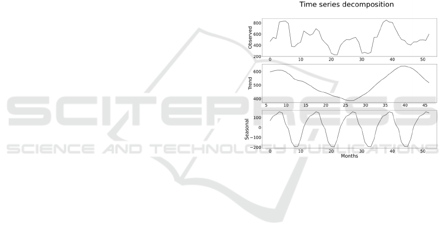
The seasonal decomposition was applied to break

down the hydropower generation time series into its

constituent components trend and seasonal. Figure 1

represents the observed time series, the detected

trend, and the seasonal pattern.

Figure 1: Decomposition of hydropower production time

series.

The trend component within a time series offers a

comprehensive view of the underlying behavior or

trajectory observed in the dataset over an extended

period. It reflects the long-term movement,

identifying whether the data generally display an

upward, downward, or relatively stable pattern over

time. An upward trend signifies consistent growth or

increase in the time series, while a downward trend

indicates a decline or decrease.

Upon close inspection of the dataset spanning

from 2019 to 2021, an evident declining trend

emerges, suggesting a consistent decrease in the

observed values over this timeframe. However, an

intriguing shift occurs thereafter, marking a reversal

in the trend. From 2021 to 2022, the dataset reflects

an increasing pattern, signifying a notable rise in

values. Subsequently, the trend reverts to a declining

trajectory, indicating a return to decreasing values.

Optimizing Planning Strategies: A Machine Learning Forecasting Model for Energy Aggregators and Hydropower Producers

495

The behavior of seasonality and trend is contingent

upon the variability of power, which in turn relies on

the fluctuating flow rate, a variable attribute owing to

its source. The flow rate fluctuates due to its origin

from the slopes of Mount Etna and is subject to the

influence of rainfall and the melting of snow. As a

result, not only does the behavior differ each month but

also across years distinguished by varying levels of

rainfall and temperatures. These factors impact the

creation and melting of snow, thereby contributing to

the variability observed over time.

Shifting the focus to the seasonal component, it

captures the recurring, periodic patterns or

seasonality inherent within the time series data. This

component reveals cyclicality or periodic fluctuations

that occur regularly within specific timeframes, such

as daily, weekly, monthly, or yearly cycles. Peaks and

troughs within the seasonal component correspond to

the high and low points recurring within each

seasonal cycle.

Notably, the seasonal pattern within this dataset

exhibits a yearly recurrence, wherein the identified

patterns tend to replicate themselves, presenting

similar characteristics and fluctuations within each

annual cycle. This seasonality can be particularly

valuable for understanding and forecasting trends tied

to specific time periods or seasons, aiding in better

predictions or analysis within seasonal contexts.

Domain experts working at Siciliacque validated

the existence of a noticeable seasonal pattern,

providing and confirming detailed insights into the

variations observed in the flow rate directed in input to

the hydropower plant. The flow rate exhibits variability

ranging from 200 l/s to 1000 l/s, peaking typically in

May or June. Subsequently, from June onward, it

steadily declines, reaching its lowest production of 200

liters in months such as September or October, before

gradually rising again toward the peak.

After the statistical analysis results, models

described in Section 3 were considered, testing

various combinations of algorithms and

hyperparameters. For each algorithm, the best-

performing model was detected. The average

performance metrics of the three models are reported

in Table 1.

The best TCN model obtained operates with the

following hyperparameters: in_len = 11, kernel_size

= 7, num_filters = 255, num_layers = 3, dilation_base

= 7, weight_norm = True, dropout = 0.4. The

hyperparameters of the best N-Beats model are in_len

= 11, num_stacks = 27, num_blocks = 2, num_layers

= 3, and dropout = 0.0. Instead, the parameters of the

top ARIMA model are p = 0, d = 0, q = 0, P = 1, D =

0, and Q = 2, with a seasonal period equal to 12.

Table 1: Average performance metrics of the three best-

performing models for each algorithm.

Metrics TCN NBEATS ARIMA

SMAPE 5.913 11.763 11.614

MAPE 5.911 11.733 11.484

RMSSE 0.674 0.737 0.805

MASE 0.896 1.034 1.12

As reported in Table 1, TCN achieved the lowest

SMAPE of 5.913, indicating better accuracy in

forecasting compared to N-Beats (11.763) and

ARIMA (11.614). Lower SMAPE values signify

better accuracy and closeness of predicted values to

the actual values. Similarly, TCN has the lowest

MAPE (5.911), showcasing superior accuracy

compared to N-Beats (11.733) and ARIMA (11.484).

TCN once again displays the lowest RMSSE (0.674),

indicating better performance in capturing both the

magnitude and relative variations in the forecasted

values compared to the actual values. N-Beats

follows with an RMSSE of 0.737, and ARIMA with

0.805. TCN demonstrates the lowest MASE (0.896),

indicating better forecasting performance concerning

the scale of the errors compared to N-Beats (1.034)

and ARIMA (1.12).

Across all four metrics, TCN consistently

outperforms N-Beats and ARIMA, showcasing

superior accuracy and precision in its predictions for

the given dataset. With regards to N-Beats and

ARIMA, the former has higher SMAPE (11.763) and

MAPE (11.733) compared to the latter (SMAPE:

11.614, MAPE: 11.484), indicating that ARIMA

performs slightly better in terms of predicting closer

values to the actual ones. At the same time, N-Beats

demonstrates a lower RMSSE (0.737) and MASE

(1.034) compared to ARIMA (RMSSE: 0.805,

MASE: 1.12), implying that N-Beats performs

slightly better in capturing the magnitude and relative

variations between forecasted and actual values.

As explained before in Section 3.4, after training

the model with a certain number of observations, the

model was tested multiple times by making

predictions for subsequent time periods while

incrementally updating the training dataset. During

each test iteration, the model generates forecasts for

the future.

In this particular case, for every step forward in

the dataset, the model produces three forecasts for the

subsequent three months. Based on the length of the

test dataset, each multi-step forecasting model was

tested nine times, each time producing three forecasts

for subsequent months, resulting in a total of 27

individual forecasts (9 test iterations multiplied by 3

forecasts per iteration).

ICEIS 2024 - 26th International Conference on Enterprise Information Systems

496

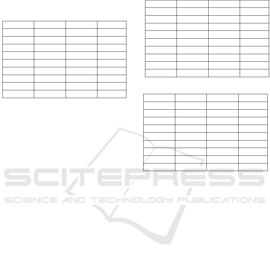
Table 2 will report more precise results regarding

the performance of the TCN model.

Table 2: SMAPE of TCN model for each test iteration.

month 2

month 3

month SMAPE

2022-07 2022-08 2022-09 5.333

2022-08 2022-09 2022-10 6.084

2022-09 2022-10 2022-11 5.483

2022-10 2022-11 2022-12 4.638

2022-11 2022-12 2023-01 8.196

2022-12 2023-01 2023-02 6.207

2023-01 2023-02 2023-03 3.239

2023-02 2023-03 2023-04 6.17

2023-03 2023-04 2023-05 7.974

As reported in Table 2, The SMAPE values range

between 3 and 8, indicating the percentage of error

between the predicted and actual values for each

forecasted three-month period. Lower SMAPE

values, such as 3.239 and 4.638, suggest higher

accuracy in prediction for those particular forecasted

periods. Most SMAPE values are below 8, suggesting

a very good overall performance in predicting

hydropower generation. Conversely, higher SMAPE

values, for instance, 8.196 and 7.974, indicate

relatively larger discrepancies between the model

predictions and the actual hydropower generation for

those periods. These occasional spikes in SMAPE

highlight potential challenges or outliers where the

model struggled to accurately predict hydropower

generation.

Therefore, the model appears to perform

relatively well in some forecasted periods,

showcasing lower SMAPE values, and indicating

higher prediction accuracy. However, certain time

intervals demonstrate higher error percentages,

suggesting challenges or limitations in accurately

forecasting hydropower generation during those

periods. Further analysis will be done to understand

the specific factors contributing to the discrepancies

observed during certain forecasted periods and to

potentially refine the model for improved accuracy

across all forecast intervals.

Table 3 and Table 4 will report more precise

results regarding the performance of the N-Beats and

the ARIMA model.

As reported in Table 3, for N-Beats moderate

SMAPE values range from 8 to 16, indicating varying

levels of forecasting accuracy across different

periods. In Table 4, SMAPE values range from 4 to

19, showing higher and lower accuracy with respect

to N-Beats in certain periods.

Table 3: SMAPE of N-Beats model for each test iteration.

month 2

month 3

month SMAPE

2022-07 2022-08 2022-09 13.717

2022-08 2022-09 2022-10 8.576

2022-09 2022-10 2022-11 10.555

2022-10 2022-11 2022-12 13.817

2022-11 2022-12 2023-01 15.810

2022-12 2023-01 2023-02 11.650

2023-01 2023-02 2023-03 15.433

2023-02 2023-03 2023-04 7.905

2023-03 2023-04 2023-05 8.401

Table 4: SMAPE of ARIMA model for each test iteration.

month 2

month 3

month SMAPE

2022-07 2022-08 2022-09 16.834

2022-08 2022-09 2022-10 19.083

2022-09 2022-10 2022-11 14.399

2022-10 2022-11 2022-12 8.733

2022-11 2022-12 2023-01 8.806

2022-12 2023-01 2023-02 7.319

2023-01 2023-02 2023-03 4.077

2023-02 2023-03 2023-04 12.191

2023-03 2023-04 2023-05 13.085

Comparing the performance results of the three

models, for the TCN model, although mostly stable,

there are minor fluctuations in SMAPE values across

different forecast intervals. Overall, this model

demonstrates relatively stable and comparatively

accurate forecasting across the periods. In N-Beats

models, while some periods exhibit higher accuracy

(e.g., the 2023-02 to 2023-04 interval), others display

comparatively higher forecasting errors (e.g., 2022-

11 to 2023-01). The accuracy of this model varies

more than the one of the TCN model, showing

fluctuations in forecasting precision. For which

regards the ARIMA model, it demonstrates higher

SMAPE values across some forecast intervals (e.g.,

the 2022-07 to 2022-10 interval), implying less

accurate predictions compared to the others.

Furthermore, it shows significant variations in error

rates among the different three-month periods.

In conclusion, this is the last ranking of models in

terms of forecasting accuracy:

 TCN, with the most consistent and accurate

predictions;

 N-Beats, showing moderate accuracy with

varying performance across different intervals;

 ARIMA, displaying higher errors.

Figure 2, Figure 3, and Figure 4 depict segments

of the observed time series spanning from September

Optimizing Planning Strategies: A Machine Learning Forecasting Model for Energy Aggregators and Hydropower Producers

497

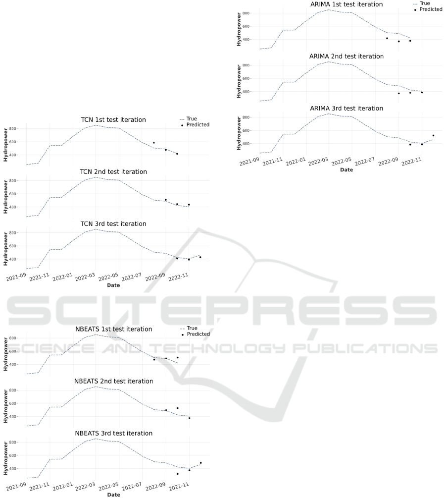
2021 to December 2022, alongside the predictions

generated by three forecasting models in their second,

third, and fourth step iterations. Specifically, the top

section of each image showcases predictions for a

three-month period spanning from August 2022 to

October 2022; the middle section displays predictions

from September 2022 to November 2022; and the

bottom section exhibits predictions from October

2022 to December 2023.

Figure 2: Observed hydropower time series and forecasts of

TCN model for the second, third, and fourth test iteration.

Figure 3: Observed hydropower time series and forecasts of

N-Beats model for the second, third, and fourth test

iteration.

Due to lack of space, a portion of the results is

displayed through images. Anyway, it is evident that

the TCN forecasts are more accurate than those of the

other models within the same time period.

Figure 4: Observed hydropower time series and forecasts of

ARIMA model for the second, third, and fourth test

iteration.

5 CONCLUSIONS

Hydropower forecasting models are fundamental for

energy aggregators and hydropower prosumers for

planning, decision-making, energy sales optimiza-

tion, and investment evaluation. Accurate forecasts

are vital for planning energy sales, maximizing

profits, and optimizing resource allocation. They

reduce risks in trading and aid grid management by

providing insights into expected supply and demand

dynamics.

This paper introduces a multi-step univariate

time-series model designed for hydropower

forecasting. The novelty of this approach lies in

employing previously unused models, such as TCN

and N-Beats, within the field of hydropower

forecasting, specifically tailored for a distinct

category of hydropower plants integrated into Water

Distribution Systems (WDSs).

To illustrate the viability of this method, the study

focuses on the Alcantara 1 Hydroelectric plant

situated in Sicily, Italy. This plant operates within a

WDS, utilizing water flow from the municipal supply

for electricity generation. The generated electricity is

then sold to the medium voltage network, securing a

favorable remuneration. This revenue significantly

mitigates the substantial costs of WDSs associated

with electricity consumption.

Following comparisons among various models,

involving a mix of complex and baseline algorithms

along with different sets of hyperparameters using a

walk-forward validation process, performance

metrics confirmed the viability of employing the TCN

ICEIS 2024 - 26th International Conference on Enterprise Information Systems

498

algorithm. Its notably high accuracy underscores its

feasibility for multi-step hydropower forecasting.

Future works involve testing and comparing

alternative machine learning algorithms while

developing different forecasting models utilizing

varied data aggregation frequencies—hourly, daily,

and weekly. Additionally, there will be evaluations of

multi-variate time series forecasting models

incorporating factors like weather measurements.

Moreover, acknowledging the existence of additional

hydroelectric plants integrated into WDSs across

various areas of Sicily, another study will be conducted

to create and compare global and local models.

ACKNOWLEDGEMENTS

Data and support were provided by Siciliacque S.p.A.

and EHT S.C.p.A. The research results presented in

this paper have been achieved inside the Water 4.0

project, named ‘Technologies for the convergence

between industry 4.0 and the integrated water cycle’.

Water 4.0 is currently running and is funded by the

Ministry of Enterprises and Made in Italy

(https://www.mimit.gov.it/en/).

REFERENCES

Adedeji, K. B., Ponnle, A. A., Abu-Mahfouz, A. M., and

Kurien, A. M. (2022). Towards Digitalization of Water

Supply Systems for Sustainable Smart City

Development—Water 4.0. Applied Sciences, 12(18),

Article 18. https://doi.org/10.3390/app12189174

Ahmad, T., Zhang, H., and Yan, B. (2020). A review on

renewable energy and electricity requirement

forecasting models for smart grid and buildings.

Sustainable Cities and Society, 55, 102052.

https://doi.org/10.1016/j.scs.2020.102052

Alhendi, A. A., Al-Sumaiti, A. S., Elmay, F. K., Wescaot,

J., Kavousi-Fard, A., Heydarian-Forushani, E., and

Alhelou, H. H. (2022). Artificial intelligence for water–

energy nexus demand forecasting: A review.

International Journal of Low-Carbon Technologies, 17,

730–744. https://doi.org/10.1093/ijlct/ctac043

ARIMA — darts documentation. (n.d.). Retrieved 16

October 2023, from https://unit8co.github.io/darts/

generated_api/darts.models.forecasting.arima.html

Arimie, C. O., Biu, E. O., and Ijomah, M. A. (2020). Outlier

Detection and Effects on Modeling. Open Access

Library Journal, 7(9), Article 9. https://doi.org/

10.4236/oalib.1106619

Bagherzadeh, F., Nouri, A. S., Mehrani, M.-J., and

Thennadil, S. (2021). Prediction of energy consumption

and evaluation of affecting factors in a full-scale

WWTP using a machine learning approach. Process

Safety and Environmental Protection, 154, 458–466.

https://doi.org/10.1016/j.psep.2021.08.040

Barzola-Monteses, J., Gómez-Romero, J., Espinoza-

Andaluz, M., and Fajardo, W. (2022). Hydropower

production prediction using artificial neural networks:

An Ecuadorian application case. Neural Computing and

Applications, 34(16), 13253–13266. https://doi.org/

10.1007/s00521-021-06746-5

Bergmeir, C., and Benítez, J. M. (2012). On the use of

cross-validation for time series predictor evaluation.

Information Sciences, 191, 192–213. https://doi.org/

10.1016/j.ins.2011.12.028

Berlotti, M., Di Grande, S., Cavalieri, S., and Gueli, R.

(2023). Detection and Prediction of Leakages in Water

Distribution Networks: Proceedings of the 12th

International Conference on Data Science, Technology

and Applications, 436–443. https://doi.org/10.5220/00

12122000003541

Borozan, D., and Pekanov Starcevic, D. (2021). Analysing

the Pattern of Productivity Change in the European

Energy Industry. Sustainability, 13(21), Article 21.

https://doi.org/10.3390/su132111742

Botchkarev, A. (2019). Performance Metrics (Error

Measures) in Machine Learning Regression,

Forecasting and Prognostics: Properties and Typology.

Interdisciplinary Journal of Information, Knowledge,

and Management, 14, 045–076. https://doi.org/

10.28945/4184

Di Grande, S., Berlotti, M., Cavalieri, S., and Gueli, R.

(2023a). A Machine Learning Approach for

Hydroelectric Power Forecasting. 2023 14th

International Renewable Energy Congress (IREC), 1–

6. https://doi.org/10.1109/IREC59750.2023.10389561

Di Grande, S., Berlotti, M., Cavalieri, S., and Gueli, R.

(2023b). A Proactive Approach for the Sustainable

Management of Water Distribution Systems:

Proceedings of the 12th International Conference on

Data Science, Technology and Applications, 115–125.

https://doi.org/10.5220/0012121200003541

Guo, J., Sun, H., and Du, B. (2022). Multivariable Time

Series Forecasting for Urban Water Demand Based on

Temporal Convolutional Network Combining Random

Forest Feature Selection and Discrete Wavelet

Transform. Water Resources Management, 36(9),

3385–3400. https://doi.org/10.1007/s11269-022-

03207-z

Hernandez-Matheus, A., Löschenbrand, M., Berg, K.,

Fuchs, I., Aragüés-Peñalba, M., Bullich-Massagué, E.,

and Sumper, A. (2022). A systematic review of

machine learning techniques related to local energy

communities. Renewable and Sustainable Energy

Reviews, 170, 112651. https://doi.org/10.1016/

j.rser.2022.112651

Herzen, J., Lässig, F., Piazzetta, S. G., Neuer, T., Tafti, L.,

Raille, G., Van Pottelbergh, T., Pasieka, M., Skrodzki,

A., Huguenin, N., Dumonal, M., Kościsz, J., Bader, D.,

Gusset, F., Benheddi, M., Williamson, C., Kosinski,

M., Petrik, M., and Grosch, G. (2023). Darts: User-

friendly modern machine learning for time series. The

Optimizing Planning Strategies: A Machine Learning Forecasting Model for Energy Aggregators and Hydropower Producers

499

Journal of Machine Learning Research, 23(1),

124:5442-124:5447.

Iria, J., and Soares, F. (2023). An energy-as-a-service

business model for aggregators of prosumers. Applied

Energy, 347, 121487. https://doi.org/10.1016/j.apen

ergy.2023.121487

Jung, J., Han, H., Kim, K., and Kim, H. S. (2021). Machine

Learning-Based Small Hydropower Potential

Prediction under Climate Change. Energies, 14(12),

Article 12. https://doi.org/10.3390/en14123643

Kerscher, S., and Arboleya, P. (2022). The key role of

aggregators in the energy transition under the latest

European regulatory framework. International Journal

of Electrical Power & Energy Systems, 134, 107361.

https://doi.org/10.1016/j.ijepes.2021.107361

Kezunovic, M., Pinson, P., Obradovic, Z., Grijalva, S.,

Hong, T., and Bessa, R. (2020). Big data analytics for

future electricity grids. Electric Power Systems

Research, 189, 106788. https://doi.org/10.1016/

j.epsr.2020.106788

Khajeh, H., Laaksonen, H., Gazafroudi, A. S., and Shafie-

khah, M. (2020). Towards Flexibility Trading at TSO-

DSO-Customer Levels: A Review. Energies, 13(1),

Article 1. https://doi.org/10.3390/en13010165

Kolbaşı, A., and Ünsal, A. (2021). A Comparison of the

Outlier Detecting Methods: An Application on Turkish

Foreign Trade Data. Journal of Mathematical Sciences,

5, 213–234.

Kostić, S., Stojković, M., and Prohaska, S. (2016).

Hydrological flow rate estimation using artificial neural

networks: Model development and potential

applications. Applied Mathematics and Computation,

291(C), 373–385.

Koutsandreas, D., Spiliotis, E., Petropoulos, F., and

Assimakopoulos, V. (2022). On the selection of

forecasting accuracy measures. Journal of the

Operational Research Society, 73(5), 937–954.

https://doi.org/10.1080/01605682.2021.1892464

Lin, K., Sheng, S., Zhou, Y., Liu, F., Li, Z., Chen, H., Xu,

C.-Y., Chen, J., and Guo, S. (2020). The exploration of

a Temporal Convolutional Network combined with

Encoder-Decoder framework for runoff forecasting.

Hydrology Research, 51(5), 1136–1149.

https://doi.org/10.2166/nh.2020.100

Lopes, M., Rocha, B., Vieira, A., Sá, J., Rolim, P., and

Silva, A. (2019). Artificial neural networks approaches

for predicting the potential for hydropower generation:

A case study for Amazon region. Journal of Intelligent

& Fuzzy Systems, 36, 5757–5772. https://doi.org/

10.3233/JIFS-181604

Marneris, I. G., Ntomaris, A. V., Biskas, P. N., Baslis, C.

G., Chatzigiannis, D. I., Demoulias, C. S., Oureilidis,

K. O., and Bakirtzis, A. G. (2023). Optimal

Participation of RES Aggregators in Energy and

Ancillary Services Markets. IEEE Transactions on

Industry Applications, 59(1), 232–243.

https://doi.org/10.1109/TIA.2022.3204863

Mite, M., and Barzola-Monteses, J. (2018). Statistical

Model for the Forecast of Hydropower Production in

Ecuador. International Journal of Renewable Energy

Research, 8.

Mosavi, A., Salimi, M., Faizollahzadeh Ardabili, S.,

Rabczuk, T., Shamshirband, S., and Varkonyi-Koczy,

A. R. (2019). State of the Art of Machine Learning

Models in Energy Systems, a Systematic Review.

Energies, 12(7), Article 7. https://doi.org/10.3390/

en12071301

N-BEATS — darts documentation. (n.d.). Retrieved 16

October 2023, from https://unit8co.github.io/darts/

generated_api/darts.models.forecasting.nbeats.html

Ngoc, T. T., Dai, L. V., and Phuc, D. T. (2021). Grid search

of multilayer perceptron based on the walk-forward

validation methodology. International Journal of

Electrical and Computer Engineering (IJECE), 11(2),

1742. https://doi.org/10.11591/ijece.v11i2.pp1742-

1751

Oliveira, P., Fernandes, B., Analide, C., and Novais, P.

(2021). Forecasting Energy Consumption of

Wastewater Treatment Plants with a Transfer Learning

Approach for Sustainable Cities. Electronics, 10(10),

Article 10. https://doi.org/10.3390/electronics10101149

Optuna: A hyperparameter optimization framework—

Optuna 3.5.0 documentation. (n.d.). Retrieved 12

December 2023, from https://optuna.readthedocs.io/en/

stable/index.html

Polprasert, J., Hanh Nguyên, V. A., and Nathanael

Charoensook, S. (2021). Forecasting Models for

Hydropower Production Using ARIMA Method. 2021

9th International Electrical Engineering Congress

(iEECON), 197–200. https://doi.org/10.1109/iEECON

51072.2021.9440293

Sari, M. A., Badruzzaman, M., Cherchi, C., Swindle, M.,

Ajami, N., and Jacangelo, J. G. (2018). Recent

innovations and trends in in-conduit hydropower

technologies and their applications in water distribution

systems. Journal of Environmental Management, 228,

416–428. https://doi.org/10.1016/j.jenvman.2018.08.078

Sharif, M. N., Haider, H., Farahat, A., Hewage, K., and

Sadiq, R. (2019). Water–energy nexus for water

distribution systems: A literature review.

Environmental Reviews, 27(4), 519–544.

https://doi.org/10.1139/er-2018-0106

Temporal Convolutional Network—Darts documentation.

(n.d.). Retrieved 16 October 2023, from

https://unit8co.github.io/darts/generated_api/darts.mod

els.forecasting.tcn_model.html

Weigel, P., and Fischedick, M. (2019). Review and

Categorization of Digital Applications in the Energy

Sector. Applied Sciences, 9(24), Article 24.

https://doi.org/10.3390/app9245350

Xu, Z., Lv, Z., Li, J., and Shi, A. (2022). A Novel Approach

for Predicting Water Demand with Complex Patterns

Based on Ensemble Learning. Water Resources

Management, 36(11), 4293–4312. https://doi.org/10.10

07/s11269-022-03255-5

Yi, S., Kondolf, G. M., Sandoval-Solis, S., and Dale, L.

(2022). Application of Machine Learning-based Energy

Use Forecasting for Inter-basin Water Transfer Project.

ICEIS 2024 - 26th International Conference on Enterprise Information Systems

500

Water Resources Management, 36(14), 5675–5694.

https://doi.org/10.1007/s11269-022-03326-7

Zhou, F., Li, L., Zhang, K., Trajcevski, G., Yao, F., Huang,

Y., Zhong, T., Wang, J., and Liu, Q. (2020). Forecasting

the Evolution of Hydropower Generation. Proceedings

of the 26th ACM SIGKDD International Conference on

Knowledge Discovery & Data Mining, 2861–2870.

https://doi.org/10.1145/3394486.3403337

Optimizing Planning Strategies: A Machine Learning Forecasting Model for Energy Aggregators and Hydropower Producers

501