Multi-Layer Energy Management System for Cost Optimization of

Battery Electric Vehicle Fleets

obinson Medina

1 a

, Nikos Avramis

1 b

, Subhajeet Rath

1 c

, Mohammed Mahedi Hasan

3 d

Dai-Duong Tran

3 e

, Zisis Maleas

4 f

, Omar Hegazy

3 g

and Steven Wilkins

1,2 h

Powertrains Department, TNO, The Netherlands

Electrical Engineerging, Eindhoven Unviersity of Technology, The Netherlands

Electrical Engineering and Power Electronics, Vrije Universiteit Brussels, Belgium

Operations Research, Centre for Research & Technology Hellas, Greece

Keywords:

Energy Management System, Battery Electric Vehicle, Smart Charging, Vehicle Speed Advise,

Vehicle Thermal Optimization, Vehicle Routing Problem.

Abstract:

One of the biggest barriers for a wider adoption of Battery-Electric Vehicles (BEVs) is their relatively higher

cost compared to their combustion-based alternatives. A potential solution is to develop Energy Management

Systems (EMSs), which make a more efﬁcient use of the vehicle energy, resulting in a cheaper operation.

EMSs are commonly composed of algorithms operating at ﬂeet and vehicle layers. For example, at ﬂeet layer

one can ﬁnd eco-routing for optimising the vehicle route, and eco-charging for smart charging. Likewise, at

vehicle layer one can ﬁnd algorithms such as eco-driving for minimizing speed-related losses and eco-comfort

for minimizing the thermal-components energy consumption. These eco-functions affect the operational cost

of the ﬂeet due to reduction of metrics such as energy consumption and travelling time (which impacts labor

costs). This paper presents the development of a multi-layer EMS, which integrates the aforementioned ﬂeet

and vehicle-level eco-functions. The paper focuses on the energy and operational cost savings that such a

multi-layer EMS can bring to a ﬂeet owner. Simulation results show that the EMS saves on costs produced by

travelling time and energy consumption. However, the ideal ratio between these savings ultimately depends

on the region, as electricity price and labor costs vary greatly.

1 INTRODUCTION

Battery-Electric Vehicles (BEVs) are currently

emerging as a viable replacement for Internal-

Combustion Engine (ICE)-based vehicles in many

transport sectors (Smith, 2010; Ewert et al., 2020).

This replacement is mostly motivated by the en-

vironmental advantages that BEVs have, such as

zero-tailpipe emissions and lower well-to-wheel

emissions (Ahmadi, 2019; Gao et al., 2023). For

some light-duty commercial applications, such as

https://orcid.org/0009-0001-2214-6153

https://orcid.org/0009-0007-3345-1018

https://orcid.org/0000-0001-8655-0334

https://orcid.org/0000-0001-7663-4948

https://orcid.org/0000-0002-3593-0748

https://orcid.org/0000-0003-1909-1259

https://orcid.org/0000-0002-8650-7341

https://orcid.org/0000-0001-9498-2321

last-mile deliveries, the current available BEVs are

already a feasible alternative for ICE (Siragusa et al.,

2022; Sendek-Matysiak et al., 2022). However,

BEVs still face multiple challenges such as increased

costs (compared to ICEs) (Anosike et al., 2023). This

challenge can be partially overcome by the usage of

Energy Management Systems (EMSs), which seek to

make the operation of BEVs more efﬁcient.

Commonly, EMSs are developed to optimize a

single aspect of the vehicle operation. Such EMSs

are found on ﬂeet or vehicle layers. For example,

when applied directly on the vehicle, one can ﬁnd al-

gorithms such as eco-comfort and eco-driving, which

are focused on reducing the on-board energy con-

sumption. Speciﬁcally, an EMS such as eco-comfort

minimizes the energy consumption of all thermal

components in the vehicle while eco-driving provides

a speed advise for the driver which minimizes the

energy consumption of the vehicle powertrain. Ex-

amples of such algorithms can be found in (Kwak

112

Medina, R., Avramis, N., Rath, S., Hasan, M., Tran, D., Maleas, Z., Hegazy, O. and Wilkins, S.

Multi-Layer Energy Management System for Cost Optimization of Battery Electric Vehicle Fleets.

DOI: 10.5220/0012627000003702

Paper published under CC license (CC BY-NC-ND 4.0)

In Proceedings of the 10th International Conference on Vehicle Technology and Intelligent Transport Systems (VEHITS 2024), pages 112-124

ISBN: 978-989-758-703-0; ISSN: 2184-495X

et al., 2023; Naeem, 2023; Medina et al., 2020).

(Kwak et al., 2023) developed an eco-comfort algo-

rithm that is based on a model predictive controller,

to achieve energy savings up to 35%. (Naeem, 2023)

designed a strategy that provides speed advise to the

driver, to maximize the BEV range and battery health.

Simulation results show energy improvements of up

to 20%. (Medina et al., 2020) co-designed an eco-

comfort and eco-driving for passenger-vehicles appli-

cations, showing that the individual savings of each

eco function (partially) adds up to up to 7.1%.

Likewise, when the EMSs are applied on a ﬂeet

layer, the algorithms focus on organizing the ﬂeet op-

erations on an efﬁcient way via algorithms such as

eco-routing and eco-charging. Eco-routing produces

vehicle routes that minimizes the traveling time of

the whole ﬂeet, while eco-charging provides a charg-

ing schedule that minimizes the total charging costs.

Examples of such algorithms can be found in (Lera-

Romero et al., 2024; Geerts et al., 2022; Zhang et al.,

2021). (Lera-Romero et al., 2024) designed an eco-

routing algorithm for last-mile deliveries which inte-

grates variability in the vehicle energy consumption

induced by the drive cycle. Simulation results show

that the scope of unfeasible problems is reduced, due

to the more precise prediction on energy consump-

tion of the algorithm. (Geerts et al., 2022; Zhang

et al., 2021) presented ﬂeet-charging strategies for

light-duty vehicles and electric busses, respectively,

which minimized the operational costs due to elec-

tricity and battery degradation.

Combinations of these ﬂeet-layer algorithms are

also common. For example, (Cataldo-D

ıaz et al.,

2024) presented a co-design of an eco-routing and

eco-charging algorithm, where the latter enables the

usage of the battery to its full capacity (i.e., 100%

instead of only the fast charging range), which in-

creases the efﬁciency of the routing problem. Like-

wise, (Lacombe, 2023) proposed a distributed opti-

mization method to combine ﬂeet-level driving strate-

gies with charging strategies (i.e., eco-driving and

eco-charging).

All of these EMSs show savings due to one or two

algorithms operating exclusively in the ﬂeet or vehi-

cle layer. Only in our technical report (Medina et al.,

2023), the energy interaction of all four mentioned

eco-functions is described. To the best of the authors

knowledge, the operational cost savings of the four

mentioned eco-functions has not been shown before.

This paper presents the interactions of multiple al-

gorithms in a multi-layer EMS for BEV ﬂeets. The

multi-layer EMS is composed of ﬂeet (eco-routing

and eco-charging) and vehicle layers (eco-driving and

eco-comfort). The resulting interactions are described

not only on the potential of energy savings, but also

in the total operational costs of using the EMS.

The remaining of this document is divided as fol-

lows. Section 2 describes the design of the multi-layer

EMS. A realistic case study is described in Section 3,

where multiple types of light-duty based deliveries

are used; Section 4 shows simulation results where

the interactions of the multi-layer EMS is analysed.

The paper closes with conclusions in Section 5.

2 MULTI-LAYER EMS DESIGN

This section presents a summary of the design of the

multi-layer EMS. The complete version of the design

can be seen in (Medina et al., 2023). The multi-layer

EMS is composed of two ﬂeet-layer algorithms (eco-

charging and eco-routing), together with two vehicle-

layer algorithms (eco-driving and eco-comfort).

2.1 Eco-Charging Algorithm

2.1.1 General Description of eco-charging

The objective of eco-charging algorithm is to gener-

ate a charging schedule for a ﬂeet of BEVs, while

reducing the charging-related costs. The charging

schedule refers to the charging power proﬁle for each

vehicle in a ﬂeet within a time window. The algo-

rithm fulﬁlls multiple objectives such as completing

the charging operation within a charging window and

reaching a target State-of-Charge (SoC) before the ve-

hicle departure while, adhering to grid/charger capac-

ity constraints.

Fig. 1 shows a schedule for a ﬂeet of N BEVs

in a charging depot, where the time-slot available for

charging is marked in green. During this window of

opportunity, vehicle i must be charged from an ini-

tial SoC (

) to a target SoC (¯z

). The output of eco-

charging algorithm is the charging power (P

) per ve-

hicle and time slot that can be drawn from the charger.

2.1.2 Mathematical Formulation of eco-charging

The complete mathematical formulation for the prob-

lem statement can be found in (Rath et al., 2023),

where the optimization problem for eco-charging is

deﬁned as

min

+ J

(1a)

s.t.

∑

i=1

≤

, ∀ j ∈ T (1b)

∈ {{0} ∪ {[

]}}

(1c)

¯z

≤ z

≤ 1, ∀ i ∈ V, (1d)

Multi-Layer Energy Management System for Cost Optimization of Battery Electric Vehicle Fleets

113

Time

Vehicle 1



Vehicle 2



Vehicle 









Vehicle N









09:00

09:15

09:30

· · ·

20:00

20:15

20:30



Figure 1: Overview of eco-charging algorithm.

The objective of Eq. 1 is to minimize the cost of

operation during ﬂeet charging. In this work, the cost

due to electricity from the grid (J

) and cost due to

battery degradation as cyclic and calendar aging (J

and J

) are considered in the objective function. Note

that there might be other charging-related costs such

as the ones related to charging losses operation or

grid-related costs (Donateo et al., 2014; Geerts et al.,

2022). Including these costs remains an open research

question.

The cost of electricity from the grid is

= E

· ε

· P

· ∆t

, (2)

where E

is the time-varying price of electricity, P

is the vector of charging power at every available

time-slot, ε

is the efﬁciency of charging from grid-

to-vehicle and ∆t

is the length of a time-slot in hours.

The battery degradation cost is given by

= E

bat

· a

· z ·10

· e

−a

0.75

e f f

, (3)

= E

bat

· b

· (P

) ·

e f f

. (4)

where E

bat

is the effective battery cost, z is the vector

of SoC at every available time-slot, T

and t are the

battery pack temperature and time elapsed for calen-

dar aging,

and Q are maximum battery capacity

and charge throughput during cyclic aging and

e f f

is the required capacity drop (normalized) after which

the battery is considered at its End-of-Life (EoL). a

and b

are battery-speciﬁc aging parameters.

Let V and T be a set of all vehicles and time-slots.

Variable

∈ P

can be deﬁned as the charge power

for vehicle i ∈ V at time-slot j ∈ T.

The optimization problem is subject to three con-

straints. Eq. 1b describes the constraint due to grid

capacity where the total power drawn by the vehicle

at every time-slot must be below the maximum power

supplied by the grid to the vehicle (

takes into

account the charging efﬁciency and scales the grid

capacity to vehicle level. Eq. 1c limits the charging

power between

and

during the charging process

while at rest it is set to 0. Here,

and

are the min-

imum and maximum charging power of the charger.

Eq. 1d constrains the vehicle SoC to reach the target

SoC without exceeding 1.

The algorithm assumes that the number of charg-

ers is equal to the number of vehicles. The charg-

ing characteristics of the battery are considered lin-

ear, i.e., the SoC increases proportionally with the

charge power. It is also assumed that the charging

window and initial and target SoC are known in ad-

vance and that a charging event cannot be interrupted

once started. Further details about the eco-charging

implementation are given in (Rath et al., 2023).

2.2 Eco-Routing Algorithm

2.2.1 General Description of eco-routing

The objective of eco-routing algorithm is to gener-

ate the optimal route that a delivery vehicle must

follow to minimize energy consumption of the ﬂeet.

The problem is constrained by battery and payload

capacity, completion of all deliveries within a stipu-

lated time and ensuring the the vehicle has adequate

charge to complete the delivery route. Such prob-

lems are deﬁned under the broader category of Vehi-

cle Route Problems (VRPs), which are computation-

ally NP-Hard (nondeterministic polynomial time). In

this work, an advanced Mixed Integer Optimization

Problem (MIP) technique (branch and cut) is used to

improve the execution time of the optimizer, as de-

scribed in (Kallehauge et al., 2005).

2.2.2 Mathematical Formulation of eco-routing

A graph G = (V, A) is deﬁned where V is the set of

stops and A is the set of Arcs (connecting the stops).

i j

, f

i j

and t

i j

are deﬁned as consumption (kWh), load

(parcels) and time (minutes) when the vehicle moves

from stop i to j. Q is the maximum capacity of the

vehicle and r time available to recharge the vehicle.

A variable x

i j

can be deﬁned as

i j

(

1, If vehicle moves from stop i to j

0, Otherwise.

The optimization problem is formulated as a VRP

with a single time window, battery and capacity con-

straints and charging operations as

min

∑

i ∈ V

∑

j ∈ V

i j

(5a)

VEHITS 2024 - 10th International Conference on Vehicle Technology and Intelligent Transport Systems

114

s.t.

∑

i ∈ V

i j

= 1, ∀ j ∈ V , i ̸= j (5b)

∑

j ∈ V

i j

= 1 ∀ i ∈ V , i ̸= j (5c)

∑

i ∈ V

0 j

≥ ⌈

/Q⌉ (5d)

∑

j ∈ V

0 j

∑

j ∈ V

(5e)

i j

≤ Qx

i j

, ∀ i ∈ V , i ̸= j (5f)

∑

j ∈ V /0

0 j

−

∑

j ∈ V /0

≥ −Q (5g)

∑

j∈V, i∈V, i̸= j

i j

≤ 480 − 30r (5h)

∑

j∈V, i∈V, i̸= j

i j

≤ 0.8 + 0.3r (5i)

∑

j∈V, i∈V, i̸= j

i j

≤| S | −1, ∀S ⊆ V /{0}. (5j)

The objective function of Eq. 5a minimizes the to-

tal energy consumption by reducing the total driven

distance. Eqs. 5b, 5c and 5e ensure that the vehicle

enters a node (request) and after dropping the order,

exits the node. Eq. 5d forces the vehicle to go to the

depot at least as many times as needed based on load

capacity constraints. Eqs. 5f and 5g ensure that the

vehicle does not exceed the capacity of the cargo body

and during every visit to the depot it can be loaded

with up to the available capacity, respectively. Eq. 5h

ensures that the total driving time and charging time

are not more than a time window of 8 hours (480 min-

utes). Similarly, Eq. 5i ensures that the SoC at the

start of the route and the additional charging that may

be performed during the day are enough to complete

the route. Finally, Eq. 5j is the subtour elimination

constraint. Subtours are paths that visit a subset of

nodes, without circling back to the depot.

2.3 Eco-Driving Algorithm

2.3.1 General Description of eco-driving

The goal of the eco-driving algorithm is twofold: ﬁrst,

to provide a speed advice to the driver and second to

provide eco-comfort with a prediction of the traction

power consumption for a certain period ahead.

The eco-driving algorithm uses an ofﬂine heuris-

tic way to determine the maximum acceleration and

deceleration of the vehicle. Using an ofﬂine heuristic

eases implementation, as it does not require a power-

ful computational platform or online data connectivity

for prediction information. However, as all the data is

precomputed, changes along the drive cycle result in

suboptimal solutions.

The heuristic algorithm generates a smooth speed

proﬁle without high power peaks, which leads to en-

ergy savings (Han et al., 2019; Ajanovi

c et al., 2018).

Additionally, the maximum speed of the vehicle is

limited to further obtain energy savings, which is spe-

cially relevant in an urban environment.

Figure 2: Optimal and regular driving speed limits.

However, these rules result in an increased travel-

ling time for the BEV, creating a trade-off is between

energy savings and travelling time. Fig. 2 shows an

example of how the speed limits are adjusted due to

eco-driving and also how the acceleration proﬁle is

affected.

2.3.2 Mathematical Formulation of eco-driving

The inputs from eco-driving include a vector of coor-

dinates with latitude and longitude (

⃗

φ,

⃗

λ) and a vec-

tor of speed limits ⃗v

lim

along the upcoming trip. An

overview of eco-driving can be seen in Fig. 3. Eco-

driving uses these inputs to create an optimal speed

proﬁle ⃗v

opt

, following the next steps:

1. Create a distance proﬁle

⃗

∆

per input coordinate.

Each point in distance vector ∆

d,i

is calculated us-

ing the Haversine formula:

∆

d,i

=2rsin

−1

sin



∆φ



cos(φ

)cos (φ

i+1

)cos



∆λ



0.5

(6)

where r is the Earth radius, φ

∈

⃗

φ , ∆λ

= λ

i+1

−

, and ∆φ

= φ

i+1

− φ

, with i = [1,. ... ,|

⃗

φ|].

⃗



Energy savings

Travelling time

Trade-off

,

⃗



Maximum speed

Acceleration limit









,





Optimize speed

Prediction matrix

Figure 3: Eco-driving topology overview.

Multi-Layer Energy Management System for Cost Optimization of Battery Electric Vehicle Fleets

115

2. An acceleration vector ⃗a

tmp

is computed using

the kinematics equation a

tmp,i

lim,i+1

−v

lim,i

2∆

d,i

, with

tmp,i

∈⃗a

tmp

, v

lim,i

∈⃗v

lim

and i = [1,. ... ,|⃗a

tmp

|].

3. A new acceleration vector ⃗a is computed using an

acceleration limit

a. That is, a

= max(a

tmp,i

,a),

= min(a

tmp,i

,−a), with a

∈⃗a.

4. An intermediate velocity vector

⃗

int

, is calculated

using ⃗a and the kinematic equation from step 2.

5. A velocity vector

⃗

f in

is computed by limiting

⃗

int

to speeds up to V , i.e., V

f in,i

= max(V

int,i

,V ) with

f in,i

∈

⃗

f in

6. A duration vector

⃗

t is created using the kinematic

equation ∆t

= 2∆

/(V

f in,i+1

f in,i

), where t

i−1

+ ∆t

and t

∈

⃗

7. The energy requirements of the drive cycle are then

computed. To do so, the traction force F

is com-

puted using:

ρc

f in,i

+ c

mgcos(α) + mgsin(α) + ma

(7)

where ρ, c

, A

, c

, m and α are the air density,

air drag, frontal area, rolling resistance, vehicle

mass and road grade, respectively. The traction

power

⃗

tr,pred

and energy

⃗

tr,pred

are computed as:

⃗

tr,pred

= F

⃗v

f in

⃗

tr,pred

⃗

tr,pred

dt. (8)

8. Using E

tr,pred

and

⃗

t, the trip energy consumption

and traveling time can be evaluated. In case they

are not satisfactory, steps 3-7 are to be recomputed

using new values for a and v. A satisfactory result

depends on the particular use case, as it will be

shown in Section 3.3. Once the result is satisfac-

tory, the optimal speed vector is deﬁned as

⃗

opt

⃗

f in

⃗

opt

then is used as speed setpoint for the driver v

st p

which is updated during the drive cycle.

2.4 Eco-Comfort Algorithm

2.4.1 General Description of eco-comfort

The eco-comfort algorithm provides temperature set-

points for the thermal systems of the vehicle, namely

the cabin, refrigerated cargo (if applicable) and the

battery pack. To reduce execution time and guar-

antee an optimal solution, the algorithm uses con-

vex models for all energy-consuming vehicle compo-

nents. Additionally, the algorithm leverages weather

forecast data, as well as the traction power proﬁle es-

timated in eco-driving, to minimize the energy con-

sumption of the thermal systems over a time horizon.

48V Battery









ℎ



Cabin





ℎ







Battery Thermal



𝑏

ℎ

𝑏



𝑏

Refrigerated Body





ℎ







Motor

ℎ













𝑏













Driven

wheels

Figure 4: Eco-comfort topology overview.

2.4.2 Mathematical Formulation of eco-comfort

The vehicle components that consume electrical en-

ergy are ﬁrst deﬁned. The basic modelling principle

is described by the power exchange among such com-

ponents. Fig. 4 shows this power exchange.

The system consists of energy buffers (x) and

power converters (h). Node A represents the inter-

connection for subsystems in the electrical power do-

main, e.g., the high-voltage bus. The sub indexes

M =

{

bat,rb,cab,bth, em

}

describe the subsystems

of the vehicle: the battery (bat), cabin (cab), refrig-

erated body (rb), electric motor (em) and the thermal

system of the battery (bth).

To formulate a convex optimization problem, the

relationship between an input (u

) and output (y

)

power in each subsystem, which represents the power

losses, is written in a quadratic form:

+ f

+ e

= 0, (9)

with m ∈ M , q

, f

and e

are parameters.

The following states are deﬁned: x

bat

is the battery

charge, while x

, x

cab

and x

bth

are the stored thermal

energies in the refrigerated body, further described as:

n,k+1

= A

n,k

+ B

n,k

+ B

d,n

n,k

, (10)

where n ∈

{

bat,rb,cab,bth

}

, A

, B

and B

d,n

, are

the state, input and input disturbance matrices, d

n,k

disturbance, k is the time instant index.

The objective of the optimization is to reduce bat-

tery energy consumption, while preserving passenger

thermal comfort. The objective function is deﬁned as:

min

n,k

∑

k∈K

bat,k

+ w



cab

− T

cab,sp



(11a)

+ w



− T

rb,sp



+ w



bth

− T

bth,sp



s.t. X

n,k+1

= A

n,k

+ B

n,k

+ B

d,n

n,k

(11b)

X ≤ X

≤ X (11c)

U ≤ U

≤ U (11d)

cab,k

+ y

bth,k

+ y

rb,k

+ y

em,k

+ y

bat,k

= 0 (11e)

m,k

+ f

m,k

+ e

m,k

≤ 0. (11f)

VEHITS 2024 - 10th International Conference on Vehicle Technology and Intelligent Transport Systems

116

With T denoting temperature and the subscript sp in-

dicating a setpoint.

In the cost function, Eq. 11b corresponds to the

previously deﬁned ﬁrst-order dynamics for each sub-

system. The capital letters in states, inputs and distur-

bances (i.e., X,U and D) indicate the aggregated sub-

systems over the time horizon. Eqs. 11c and 11d de-

note constraints on upper and lower bounds for states

(X,X ) and inputs (U,U ). The power interconnection

at node A of Fig. 4 is captured in Eq. 11e. Finally, the

quadratic relationship of Eq. 9 is captured in Eq. 11f.

Notice that Eq. 11f has been relaxed to an inequality

to ensure convexity.

The weighing factors w

-w

are calibrated heuris-

tically, to obtain energy savings while keeping cabin

in an acceptable range for the passenger.

3 CASE STUDY

This section presents a motivational case study, where

the multi-layer EMS is applied.

3.1 Vehicle Fleet

A ﬂeet of 11 BEVs is considered, to carry out dif-

ferent delivery routes, under multiple weather con-

ditions, and create a realistic operation for evaluat-

ing the multi-layer EMS. To do so, each one of the

vehicles drives one test case with a different route,

weather conditions or settings for eco-comfort. An

overview of the test cases is shown in Table 1.

The ﬂeet of vehicles is assumed to be carrying out

simultaneously two types of last-mile delivery oper-

ations: post-delivery and food-delivery case. Both

last-mile deliveries are performed out in city environ-

ments. All deliveries are carried out during day time

while all charging is carried out during nighttime. The

post-delivery test case is assumed to be carried out

in 3 different routes across Belgium. Such deliver-

ies show frequent stops to deliver packages, and the

weather conditions vary around 5

◦

C. An example of

the prediction data is shown in Fig. 5. The low-speed

instances (i.e., when the speed is less than 10 km/h)

denote delivery locations.

The food-delivery use case is executed in Thes-

saloniki, Greece. An example of the prediction data

on this use case is shown in Fig. 6. It can be seen

that the delivery of food requires fewer stops than

those of the post. Likewise, due to the location, the

weather conditions show relatively warmer tempera-

tures (above 30

◦

C) compared to post-delivery oper-

ation. These differences in weather conditions are

taken to show the difference between winter and sum-

09:00 09:10 09:20 09:30

Time Feb 10, 2022

5.8

5.9

°C

Temperature forecast

0 5 10 15

Distance [km]

[km/h]

Speed limit

Figure 5: Prediction data example of test case 12. Data

obtained using the APIs described in (Medina et al., 2023).

08:00 08:30 09:00 09:30 10:00 10:30

Time Jul 25, 2022

°C

Temperature forecast

0 10 20 30 40 50 60 70

Distance [km]

[km/h]

Speed limit

Figure 6: Prediction data example of test case 2. Data ob-

tained using the APIs described in (Medina et al., 2023).

mer operations. Note that last-mile delivery is spe-

cially relevant for the multi-layer EMS, as the re-

quired frequent stops in the city environment gives

ample opportunity for route and energy consumption

optimization. Other use cases with similar opportuni-

ties might also be of interest.

3.2 Vehicle Modelling

To evaluate the energy consumption for every test

case deﬁned in the previous section, a vehicle model

and a powertrain model are created. The models

correspond to an N1-category BEV, which is com-

monly used for urban deliveries. Such models fol-

low forward-facing dynamics, as shown for exam-

ple in (Medina et al., 2020). The model parameters

are adapted for an N1-category vehicle. The vehicle

and powertrain models are operated by a driver model

which is a controller that follows a reference speed.

Such a reference is taken as the road speed limit or

the advised speed from eco-driving.

Multi-Layer Energy Management System for Cost Optimization of Battery Electric Vehicle Fleets

117

Table 1: Test cases description.

ID Location Goal

2 Greece Summer thermal savings, passenger comfort setting 1, benchmark cabin temp at 20°

3 Greece Summer thermal savings, passenger comfort setting 2,benchmark cabin temp at 20°

4 Greece Summer thermal savings, passenger comfort setting 3, benchmark cabin temp at 20°

5 Greece Summer thermal savings, passenger comfort setting 1, benchmark cabin temp at 22°

6 Greece Summer thermal savings, passenger comfort setting 2, benchmark cabin temp at 23°

7 Greece Summer thermal savings, passenger comfort setting 3, benchmark cabin temp at 23°

8 Belgium 1 Winter thermal savings, passenger comfort setting 1, benchmark cabin temp at 20°

9 Belgium 1 Winter thermal savings, passenger comfort setting 2, benchmark cabin temp at 20°

10 Belgium 1 Winter thermal savings, passenger comfort setting 3, benchmark cabin temp at 20°

11 Belgium 2 Eco-comfort validation, passenger comfort setting 2

12 Belgium 3 Eco-driving energy savings in urban environment

3.3 Simulation Environment

To quantify the multi-layer EMS beneftis, a simula-

tion environment is designed in Matlab (Medina et al.,

2023). The simulation environment splits the problem

into online and ofﬂine parts, as Fig. 7 shows.

The ofﬂine part runs the ﬂeet-layer eco-functions

(eco-charging and eco-driving) to generate charge

planning and driving routes for the whole ﬂeet. The

eco-functions take inputs from the logistic assign-

ment, such as delivery locations or required SoC at the

start of the day. Given the generated routes and charg-

ing schedule, APIs are used to predict trafﬁc infor-

mation (e.g., the speed limit, road grade) and weather

forecast (e.g., temperature forecast) along the traveled

routes of the vehicle (see for example Fig. 6).

The online part runs a vehicle model while taking

as input the output of the ofﬂine part. For example,

the road grade affects the vehicle dynamics, and the

temperature forecasts the thermal losses. Likewise,

eco-driving and eco-comfort run in the online part.

For each time step in the simulation, the temperature

setpoints and speed advice are provided for the vehi-

cle models to follow. The resulting relevant metrics

are recorded (e.g., traveling time, energy consump-

tion) and used to evaluate the EMS performance.

3.4 Performance Metrics

The multi-layer EMS is compared using two relevant

metrics: energy consumption and total cost of oper-

ation. Energy consumption is recorded directly from

the battery and normalized for the number of traveled

kilometers along that route. Note that the on-board

eco-functions are designed to minimize this metric.

The total operational costs are considered as the

result of energy prices, labor, and battery degradation,

i.e.:

C = J

+ J

, (12)

Veh. Signals

Route

details

Weather

forecast Traffic

prediction

Route

Speed advise

Thermal

components

setpoints

Eco-charging

and charger

simulation

Base vehicle (models)

and driver model

Eco-driving

Eco-routing and

logistics information

Test case

selection

Weather and

traffic prediction

(APIs)

Power prediction profile

Eco-comfort

Online simulation

Offline simulation

Figure 7: Simulation environment overview.

where C is the total cost in [C], J

is the electricity

cost deﬁned in Eq. 2, J

and J

are the calendar and

cyclic ageing of the battery, respectively, further de-

ﬁned in Eqs. 3 and 4, and J

the labour cost given by

= T

, (13)

where T

is the total traveling time along the route and

is the driver hourly rate in [C/hour].

To compare the performance of each eco-function,

a benchmark simulation is run. For eco-routing the

benchmark corresponds to running the same logistic

assignment based on a commonly-used heuristic algo-

rithm that solves a Traveling Salesman Problem. For

eco-charging, the benchmark corresponds to applying

a greedy charging strategy (i.e., charge as soon as ar-

rival to the depot). For the on-board eco-functions,

the benchmark corresponds to running the routes pro-

vided by eco-routing, while not using the output of the

on-board eco-functions. That is, the driver follows the

speed limit, while the thermal systems follow a ﬁxed

temperature setpoint.

To compare the improvements achieved by the

multi-layer EMS, the increase or decrease of cost is

calculated as

∆C =

benchmark

− C

EcoFun

benchmark

100 [%], (14)

VEHITS 2024 - 10th International Conference on Vehicle Technology and Intelligent Transport Systems

118

where C

benchmark

and C

EcoFun

are the operational

costs [ C] related to the benchmark and eco-functions

scenarios, respectively, and ∆C is the percentage of

increase/decrease in total operational costs.

3.5 Multi-Layer EMS Parameters

To quantify the performance of the multi-layer EMS,

some parameters need to be assumed.

For eco-driving, the maximum vehicle accelera-

tion without the eco-function (i.e., in the benchmark

scenario) is taken as a = 0.66m/s

from (Purnot et al.,

2021). Therefore, maximum acceleration proﬁle with

eco-driving is assumed as a = 0.37m/s

in test cases

2-11, and a = 0.25m/s

in test cases 11 and 12.

In eco-comfort, the weight factors w

-w

are cho-

sen to give several saving settings: setting 1 corre-

sponds to an “aggressive” proﬁle (highest savings),

setting 2 to a “moderate” one (middle savings) and

setting 3 to a “smooth” one (lowest savings, maxi-

mum passenger comfort).

For eco-charging, the electricity price E

is 0.335 [C/kW h] from 23:00 to 07:00, and

0.385 [C/kW h] for the rest (Rath et al., 2023).

For the cost evaluation, the prices of labour rates

are assumed as

= 20



hour



. (15)

This price falls within the range of labour cost

in the European Union (European Comission, 2022).

Notice that driver costs has more weight than those of

electricity in the total cost calculation, as every saved

hour accounts for much more than every kW h saved.

4 SIMULATION RESULTS

This section presents the results of simulating the

multi-layer EMS with the case study of Section 3.

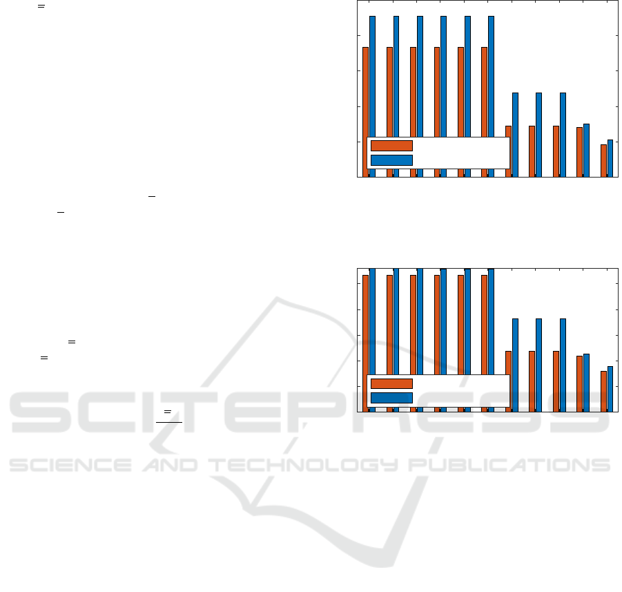
4.1 Fleet-Layer Savings of

Eco-Functions

Eco-routing is applied for case study of Section 3,

where the algorithm was able to compute a feasible

route for each one of the test cases. As discussed in

Section 2.2, the main goal of the algorithm is to re-

duce the total traveling distance. This is shown in

Fig. 8 where the optimized traveling distance is al-

ways lower than the benchmark. The improvement is

mostly visible in the test cases 8 to 10, as these re-

late to post-delivery cases which has a higher density

Eco-routing travelled distance

2 3 4 5 6 7 8 9 10 11 12

Trip ID

100

Travelled distance [km]

With eco-routing

Without eco-routing

Figure 8: Travelled distance comparison with eco-routing.

2 3 4 5 6 7 8 9 10 11 12

Trip ID

100

Travelled time [min]

With eco-routing

Without eco-routing

Eco-routing results overview

Figure 9: Travelled time comparison with eco-routing.

of deliveries compared to food-delivery. This creates

more optimization opportunities for the parcel order.

Using the simulation environment proposed in

Section 3.3, the proposed routes are simulated for

different test cases without enabling on-board eco-

functions. The resulting traveling times are shown in

Fig. 9. As expected, the traveling time is shorter due

to the shorter routes, which results in a reduction of

operational costs, as subsequent paragraphs show.

Using the energy requirements provided by eco-

routing, the eco-charging algorithm is run on the en-

tire ﬂeet. The resulting charged energy is seen in

Fig. 10. Note that the charged energy while using

eco-charging, already includes the effects of using

eco-driving and eco-comfort. Therefore, using eco-

charging results in less energy needed to be charged

to each vehicle in the ﬂeet.

Considering that the cost function of eco-charging

reduces the total charging-related costs, the beneﬁts

of this algorithm are reﬂected in the economic sav-

ings. This is shown in Table 2. Due to the vari-

able electricity price, eco-charging tends to charge

the ﬂeet when the energy price are lower. Likewise,

Multi-Layer Energy Management System for Cost Optimization of Battery Electric Vehicle Fleets

119

Eco-charging comparison

2 3 4 5 6 7 8 9 10 11 12

Trip ID

Charged energy [kWh]

Without eco-charging

With eco-charging

Figure 10: Charged energy comparison with eco-charging.

Table 2: Cost savings from eco-charging.

Benchmark [C] Eco-charging [C] [%]

ID J

∆C

2 5.7 2.2 2.2 3.25 0.96 1.48 43.9

3 5.7 2.2 2.0 3.31 0.98 1.39 43.1

4 5.7 2.2 2.2 3.34 1 1.46 42.9

5 5.6 2.1 2.0 3.25 0.96 1.4 43.1

6 5.6 2.1 2.2 3.31 0.98 1.46 42.6

7 5.6 2.1 2.0 3.34 1 1.38 42.1

8 2.5 0.6 2.0 1.34 0.25 1.82 34.7

9 2.5 0.6 1.8 1.44 0.28 1.68 32.9

10 2.5 0.6 1.9 1.47 0.29 1.73 32

11 2.1 0.5 1.7 1.61 0.33 1.52 21.5

12 1.4 0.2 1.6 1.09 0.19 1.52 18.4

using the insights of the aging model on the battery,

the algorithm achieves less deterioration in the battery

lifetime compared to the benchmark strategy. This

is more signiﬁcant in terms of cyclic aging J

, as it

seems to have a larger impact on the battery lifetime.

This reduction corresponds to a reduction of at least

20% of costs in all test cases.

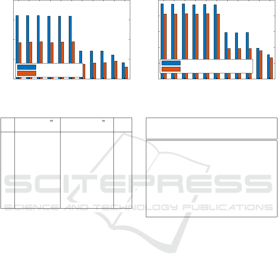
A total cost comparison of the cloud-based eco-

functions is shown in Fig. 11. The total operational

costs are always lower. Note that the electricity cost

is not taken into account in Fig. 11, as this is the

result of the combined effect of using the on-board

eco-functions and eco-charging. The electricity cost

is therefore going to be considered in the on-board

eco-functions, in the next subsection.

4.2 Vehicle-Layer Savings of

Eco-Functions

Using the vehicle model of Section 3.2, the routes

provided by eco-routing, and the trafﬁc and weather

prediction information provided by the APIs de-

scribed in Fig. 7, the onboard eco-functions are tested

Cloud functions cost comparison

2 3 4 5 6 7 8 9 10 11 12

Trip ID

Cost [€]

Without eco-functions

With eco-charging and eco-routing

Figure 11: Cost comparison with ﬂeet layer eco-functions.

Table 3: On-board energy consumption in [kW h/km].

ID No eco-

functions

With eco-

driving

With eco-

comfort and

eco-driving

2 0.137 0.135 0.126

3 0.137 0.135 0.128

4 0.137 0.135 0.129

5 0.133 0.131 0.126

6 0.133 0.131 0.128

7 0.133 0.131 0.129

8 0.149 0.145 0.13

9 0.149 0.145 0.14

10 0.149 0.145 0.143

11 0.188 0.165 0.163

12 0.197 0.169 0.166

on each one of the case studies of Table 1. As de-

scribed in Section 2, the onboard eco-functions min-

imize energy consumption while driving the vehicle.

An overview of the energy savings is shown in Ta-

ble 3. Note that in each one of the trips, the energy

consumption per kilometer is lower than while driv-

ing without using the eco-functions.

For the case of eco-comfort, although it produces

savings on all cases, the largest savings appears un-

der setting 1 (aggressive), which corresponds to test

cases 2, 5, and 8. The lowest savings corresponds to

setting 3 (smooth), which are cases 4, 7 and 10. Ta-

ble 3 also shows relatively larger savings during win-

ter than during summer. See for example the savings

of test case 2 (summer) and test case 8 (winter). These

larger savings are due the vehicle being equipped with

an air conditioning for cooling and an electric resis-

tance for heating. An air conditioning requires less

energy to create the same difference in temperature

than a resistor due to its Coefﬁcient of Performance,

resulting in more saving possibilities during winter.

Note that eco-comfort does not affect traveling time

VEHITS 2024 - 10th International Conference on Vehicle Technology and Intelligent Transport Systems

120

as it does not inﬂuence the driving dynamics.

Eco-driving provides the largest amount of sav-

ings in test cases 11 (12%) and 12 (14%), compared

to the rest of the test cases (on average 2.9%). This is

because in the test cases 11 and 12, the speed advice

is built with the extra saving setting for limiting the

acceleration, in contrast with the acceleration of the

other test cases. This test case shows the large poten-

tial of energy savings that eco-driving has.

However, the energy savings produced by eco-

driving come at the cost of extra traveling time, as

shown in Fig. 12, which increases the labor costs. For

example, test case 12 increases the traveling time by

25.9%, while the rest of the test cases increase it by

on average 8.2%. This creates a trade-off between the

savings on energy and the ones on labor: larger sav-

ings on energy result in added traveling time which

creates labor costs. The acceleration limit and maxi-

mum speed of eco-driving need to be carefully chosen

for each particular test case, to provide total opera-

tional savings.

2 3 4 5 6 7 8 9 10 11 12

Trip ID

100

120

Travelled time [min]

With eco-driving

Without eco-driving

Travelled time comparison

Figure 12: Travelled time comparison of eco-driving.

Using the rates presented in Section 3.5, the costs

presented in Fig. 13 are calculated. Note that despite

the combined energy savings of eco-comfort and eco-

driving, the total operational cost per test case is virtu-

ally the same in most test cases, except for test cases

11 and 12. This is because the extra traveling time

produced by eco-driving is canceling the effect of the

energy savings, due to the driver rates being more sig-

niﬁcant than the electricity price. This is also partially

because the charging operation occurs with low elec-

tricity prices, which is a result of using eco-charging.

Notice that in test cases 11 and 12, the total cost of

the eco-functions remains higher than the benchmark,

because eco-driving produces signiﬁcantly more trav-

eling time. Eco-driving could become cost-effective

if the electricity price is comparable to driver rates or

eco-driving is tuned to reduce traveling time, which

is likely to result in higher energy consumption. The

former is brieﬂy shown in the next subsection. The

latter only requires the driver to accelerate as fast as

possible, which neglects the need for speed advice.

On-board functions cost comparison

2 3 4 5 6 7 8 9 10 11 12

Trip ID

Cost [€]

Without eco-functions

With eco-driving and eco-comfort

Figure 13: Cost comparison with onboard eco-functions.

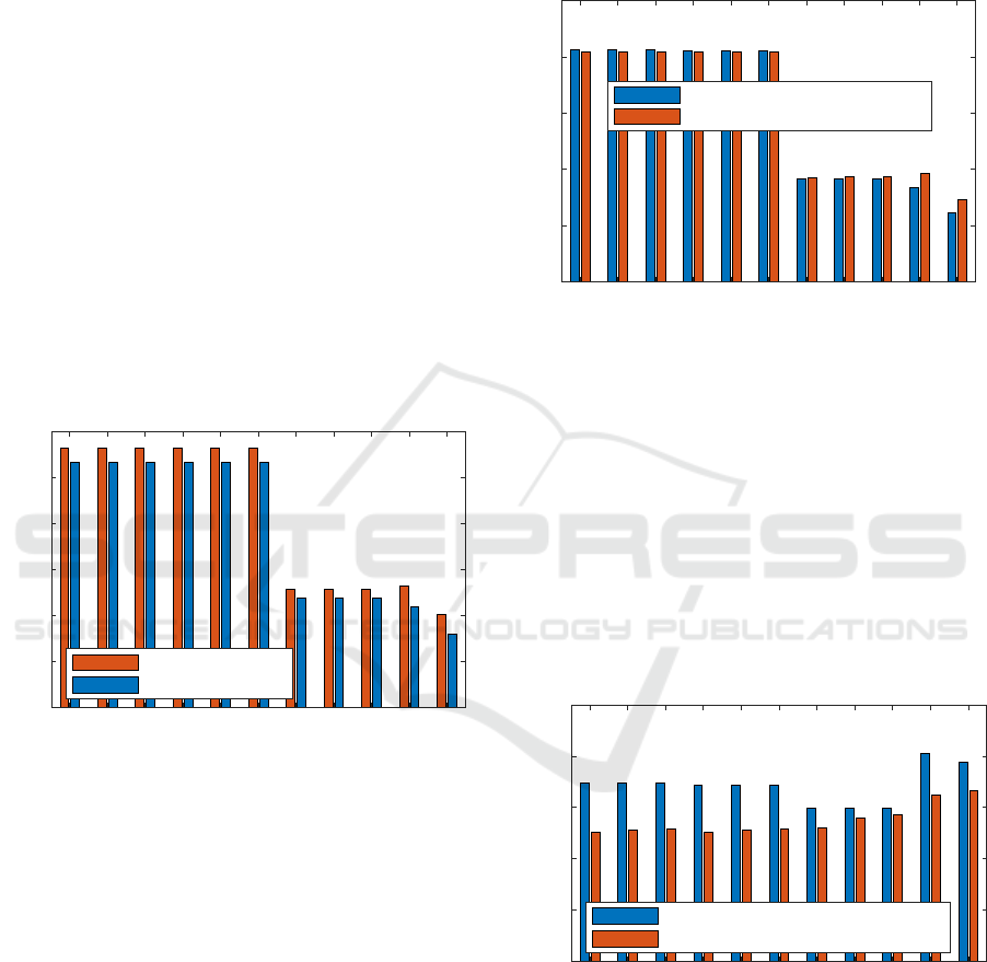
4.3 Combined Savings Effect of the

Multi-Layer EMS

The energy consumption of the complete multi-layer

EMS is presented in Fig. 14. Note that in this case, the

benchmark corresponds to not using any eco-function

while driving the benchmark routes. Using the multi-

layer EMS reduces the energy consumption in all the

test cases. This is mostly due to the effect of the on-

board eco-functions.

2 3 4 5 6 7 8 9 10 11 12

0.05

0.1

0.15

0.2

0.25

Energy consumption [kWh/km]

Without ecos

With eco-routing, -driving and -comfort

Difference in energy savings

Figure 14: Energy consumption comparison with all eco-

functions.

The traveling time comparison is shown in Fig. 15.

As the ﬁgure shows, the traveling time is virtually the

same in test cases 2-7, signiﬁcantly shorter in 8-10

and longer in 11-12. This traveling time is the result

of the shorter routes produced by eco-routing and the

longer traveling time produced by eco-driving. Note

that the total traveling time is only larger in test cases

Multi-Layer Energy Management System for Cost Optimization of Battery Electric Vehicle Fleets

121

11 and 12, where eco-driving increases it.

2 3 4 5 6 7 8 9 10 11 12

Trip ID

100

120

Travelled time [min]

Without ecos

With eco-routing, -driving and -comfort

Difference in travelled time

Figure 15: Travelled time comparison with all eco-

functions.

Table 4 shows an overview of the resulting opera-

tional costs of using the multi-layer EMS. In most of

the cases, the total operational costs are lower using

the eco-functions, despite the added cost of the eco-

driving in the vehicle layer. Following the trend of

Fig. 15, the costs on test cases 11 and 12 are higher,

due to the additional traveling induced by eco-driving.

Table 4: Cost improvement based on Eq. 14 and the costs

of Section 3.5. Positive values indicate savings.

ID On board only Fleet only Combined

2 1.04 9.35 5.23

3 0.89 9.15 5.04

4 0.82 9.3 5.09

5 0.87 8.44 4.67

6 0.72 8.62 4.69

7 0.65 8.39 4.53

8 -0.63 33.48 19.66

9 -1.18 33.47 19.38

10 -1.34 33.45 19.32

11 -14.72 5.28 -4.55

12 -19.64 10.6 -3.53

To show more signiﬁcant savings of the multi-

layer EMS, the operational costs are re-calculated

using a hypothetical labor cost of C

= 2[C/hour],

while the electricity costs are kept the same. The re-

sults are summarized in Table 5. With this reduced

rate, the battery degradation and electricity price be-

come more signiﬁcant in the cost calculations. For

example in the cloud functions costs, battery degra-

dation becomes the dominant factor with the reduced

hourly rate, making the relative savings higher than

with a normal hourly rate. Likewise, in the on-board

functions costs, electricity price becomes the domi-

nant factor, yielding to savings in all test cases. Con-

sequently, the multi-layer EMS shows costs and en-

ergy savings in all test cases. This hypothetical rate

shows that the multi-layer EMS can be cost-effective,

depending on the ratio of labor and electricity prices.

Table 5: Cost improvement based on Eq. 14 and C

= 2

[C/hour]. Positive values indicate savings.

ID On board only Fleet only Combined

2 24.29 26.78 25.46

3 23.64 26.1 24.78

4 23.32 26.53 24.83

5 23.72 25.66 24.62

6 23.06 26.23 24.55

7 22.74 25.41 23.98

8 25.42 28.8 27.3

9 22.98 28.57 26.05

10 22.25 28.52 25.71

11 7.08 12.01 9.59

12 4.39 11.55 8.34

5 CONCLUSIONS

This paper presented the operational cost and energy

savings of a multi-layer Energy Management System

(EMS) for a ﬂeet of Battery-Electric Vehicle (BEV),

used in distribution logistics.

The EMS is composed of ﬂeet-layer (eco-routing

and eco-charging) and vehicle-layer algorithms (eco-

driving and eco-comfort). Eco-routing ﬁnds the route

for the vehicles in the ﬂeet, which minimizes the to-

tal traveling distance. Eco-charging ﬁnds a charging

schedule, which minimizes battery degradation and

electricity cost. Eco-driving provides each driver with

a speed advise, that minimizes the energy consump-

tion of the vehicle powertrain. Eco-comfort mini-

mizes the energy consumption of the vehicle ther-

mal systems, while considering driving comfort. The

multi-layer EMS is tested in a case study, which sim-

ulates information about the operation of a ﬂeet of

BEVs using real trafﬁc and weather information.

Simulation results show that on a ﬂeet level, eco-

routing reduces the traveling distance of the whole

ﬂeet when compared to a baseline algorithm. This in

turn reduces the labour related costs due to the faster

delivery times. Eco-charging reduces the charging-

related costs because the charging operation mostly

occurs when the electricity tariffs are low and be-

cause the reduced battery degradation. Both ﬂeet-

level eco-functions add their individual savings to the

total ﬂeet-level savings.

Results also show that eco-comfort reduces the en-

ergy consumption of the thermal systems on the ve-

VEHITS 2024 - 10th International Conference on Vehicle Technology and Intelligent Transport Systems

122

hicle, depending on several factors, such as ambient

temperature and algorithm settings. All energy sav-

ings of eco-comfort result in savings on operational

costs, with a possible reduction in thermal comfort.

Eco-driving also reduces the energy consumption of

the vehicle powertrain, depending on the maximum

acceleration set in the algorithm and the maximum

speed. However, such a reduction comes with an

additional traveling time, which increases the labor

costs. The settings of eco-driving needs to be care-

fully chosen depending on the electricity price and the

labor costs, to provide operational savings.

Lastly, results also show that using all the eco-

functions in the multi-layer EMS results in a reduc-

tion in energy consumption in the entire ﬂeet. How-

ever, the operational cost savings related to energy

consumption are slightly reduced by the fact that eco-

charging charges the ﬂeet preferably when the elec-

tricity prices are lower. Likewise, the traveling time of

each vehicle is increased by the effect of eco-driving

and decreased by the effect of eco-routing. The ben-

eﬁts of these eco-functions can cancel each other if

eco-driving is not properly tuned, leading to higher

labour costs. Therefore, an additional simulation is

run to show a hypothetical case in which the beneﬁts

of both eco-driving and eco-routing can be added to

each other, due to the costs of energy-related savings

being comparable to the labor-related savings.

ACKNOWLEDGEMENTS

This research has received funding from the European

Union’s Horizon 2020 research and innovation pro-

gramme under grant No 101006943, title of URBAN-

IZED.

REFERENCES

Ahmadi, P. (2019). Environmental impacts and behav-

ioral drivers of deep decarbonization for transporta-

tion through electric vehicles. Journal of Cleaner Pro-

duction, 225:1209–1219.

Ajanovi

c, Z. et al. (2018). A novel model-based heuris-

tic for energy-optimal motion planning for automated

driving. 15th IFAC Symposium CTS, 51(9):255–260.

Anosike, A. et al. (2023). Exploring the challenges of elec-

tric vehicle adoption in ﬁnal mile parcel delivery. In-

ternational Journal of Logistics Research and Appli-

cations, 26(6):683–707.

Cataldo-D

ıaz, C. et al. (2024). Mathematical models for the

electric vehicle routing problem with time windows

considering different aspects of the charging process.

Operational Research, 24(1):1.

Donateo, T. et al. (2014). A method to estimate the environ-

mental impact of an electric city car during six months

of testing in an italian city. Journal of Power Sources,

270:487–498.

European Comission (2022). Hourly labour costs

ranged from C8 to C51 in the EU. https:

//ec.europa.eu/eurostat/web/products-eurostat-news/

w/DDN-20230330-3. Accessed:01-02-2024.

Ewert, A. et al. (2020). Small and light electric vehicles:

An analysis of feasible transport impacts and oppor-

tunities for improved urban land use. Sustainability,

12(19).

Gao, Z. et al. (2023). Electric vehicle lifecycle carbon

emission reduction: A review. Carbon Neutralization,

2(5):528–550.

Geerts, D. et al. (2022). Optimal charging of electric ve-

hicle ﬂeets: Minimizing battery degradation and grid

congestion using battery storage systems. In Second

International Conference SMART, pages 1–11. IEEE.

Han, J., Vahidi, A., and Sciarretta, A. (2019). Fundamen-

tals of energy efﬁcient driving for combustion engine

and electric vehicles: An optimal control perspective.

Automatica, 103:558–572.

Kallehauge, B. et al. (2005). Vehicle routing problem with

time windows. Springer.

Kwak, K. H. et al. (2023). Thermal comfort-conscious

eco-climate control for electric vehicles using model

predictive control. Control Engineering Practice,

136:105527.

Lacombe, R. (2023). Distributed optimization for the opti-

mal control of electric vehicle ﬂeets.

Lera-Romero, G. et al. (2024). A branch-cut-and-price al-

gorithm for the time-dependent electric vehicle rout-

ing problem with time windows. European Journal of

Operational Research, 312(3):978–995.

Medina, R. et al. (2020). Multi-layer predictive energy man-

agement system for battery electric vehicles. IFAC-

PapersOnLine, 53(2):14167–14172.

Medina, R. et al. (2023). Urbanized D4.4: Optimised self-

adaptive, multi-layer EMS design and virtual valida-

tion ﬂeet management algorithm. Technical report,

European Union Horizon 2020, research and innova-

tion programme.

Naeem, H. M. Y. (2023). Eco-driving Control of Electric

Vehicle with Realistic Constraints. PhD thesis, Capital

University.

Purnot, T. et al. (2021). Urbanized D2.1: Mission proﬁles,

KPIs, assessment plan, List of vehicle requirements,

design speciﬁcations and shared interfaces. Technical

report, European Union Horizon 2020, research and

innovation programme.

Rath, S. et al. (2023). Real-time optimal charging strat-

egy for a ﬂeet of electric vehicles minimizing battery

degradation. In SEFET, pages 1–8. IEEE.

Sendek-Matysiak, E. et al. (2022). Total cost of ownership

of light commercial electrical vehicles in city logis-

tics. Energies, 15(22).

Siragusa, C. et al. (2022). Electric vehicles performing last-

mile delivery in B2C e-commerce: An economic and

Multi-Layer Energy Management System for Cost Optimization of Battery Electric Vehicle Fleets

123

environmental assessment. International Journal of

Sustainable Transportation, 16(1):22–33.

Smith, W. J. (2010). Can EV (Electric Vehicles) address

Ireland’s CO2 emissions from transport? Energy,

35(12):4514–4521.

Zhang, L. et al. (2021). Optimal electric bus ﬂeet scheduling

considering battery degradation and non-linear charg-

ing proﬁle. Transportation Research Part E: Logistics

and Transportation Review, 154:102445.

VEHITS 2024 - 10th International Conference on Vehicle Technology and Intelligent Transport Systems

124