Pareto-Optimal Execution of Parallel Applications with Respect to Time

and Energy

Thomas Rauber

1 a

and Gudula R

unger

2 b

Department of Computer Science, University of Bayreuth, Germany

Department of Computer Science, Chemnitz University of Technology, Germany

Keywords:

Numerical Solution Methods, Parameter Selection, Runtime Performance, Energy Consumption.

Abstract:

Compute-Bound numerical solution methods have a high demand for computational power and, thus, for

energy. Both depend strongly on the numerical accuracy required for the approximation solution. A higher

numerical accuracy often requires more execution time and energy. However, this dependence is more subtle

and diverse. That means for a given numerical problem, different settings of the solution process, such as the

use of different solvers, different implementation variants, different numbers of cores, or different operational

frequencies result in a large number of different possibilities for the solution process, each of which may

lead to a potentially different execution time and energy consumption. The best combination also depends

on the speciﬁc execution platform used. Using different tolerance values for the time steps in the solution

process adds another degree of complexity with a potentially different accuracy of the resulting approximation

solution. The goal of this article is to investigate the selection process of performance-optimal variants of all

these computation possibilities when solving a given numerical problem. In particular, a selection process

is proposed determining Pareto-optimal computation variants of the numerical method. As representative

numerical solution method, explicit solution methods for ordinary differential equations are considered.

1 INTRODUCTION

The execution of software on computing devices con-

sumes more and more energy and it is an important

concern to reduce this energy consumption for envi-

ronmental reasons (OECD, 2023). The energy con-

sumption can be reduced by employing hardware sys-

tems that are more energy-efﬁcient or by developing

methods to execute the software in a more energy-

efﬁcient way (Brown and Reams, 2010). In this arti-

cle, the second aspect is considered in more detail.

Energy efﬁciency is especially important for

compute-intensive applications that are executed on

large parallel systems, since these applications often

use large amounts of energy (Orgerie et al., 2014).

Many compute-intensive applications come from the

area of scientiﬁc computing, especially from the nu-

merical solution of differential equations modeling

phenomena in science and engineering, including

classical physics, economy, chemistry, and engineer-

ing. In most cases, it is not possible to represent the

https://orcid.org/0000-0002-3102-6858

https://orcid.org/0000-0002-5364-2088

exact solution in closed form and, therefore, the so-

lution has to be approximated by a numerical tech-

nique. The solution of differential equations requires

the use of suitable numerical methods, which are of-

ten compute-bound and require a large amount of exe-

cution time and energy. Approximations usually pro-

duce an error due to the numerical calculations per-

formed, and it is an important concern to determine

how good the approximation ﬁts to the real solution at

the approximation points (Deuﬂhard and Hohmann,

2003). This is denoted as the accuracy of the solu-

tion. For many numerical methods, the accuracy can

be inﬂuenced by algorithmic parameters, such as tol-

erance values and error bounds that are used to decide

whether a computation step is accepted or needs be

repeated.

The execution time and energy consumption of the

execution of a numerical method strongly depends on

the execution platform and the execution parameters

that are used for the execution. Usually, the numeri-

cal method is implemented as parallel software sys-

tem and the number of execution units (processors

or cores) used for the execution has a large inﬂuence

on the execution time and energy consumption. Us-

Rauber, T. and Rünger, G.

Pareto-Optimal Execution of Parallel Applications with Respect to Time and Energy.

DOI: 10.5220/0012627100003714

Paper published under CC license (CC BY-NC-ND 4.0)

In Proceedings of the 13th International Conference on Smart Cities and Green ICT Systems (SMARTGREENS 2024), pages 65-72

ISBN: 978-989-758-702-3; ISSN: 2184-4968

ing a larger number of execution units often reduces

the execution time until a certain saturation point is

reached, which depends on the algorithmic structure

and parallel implementation of the numerical method.

However, the energy consumption may exhibit a dif-

ferent characteristic of the growth behavior depending

on the amount of parallelism. Different selections of

execution parameters may lead to the smallest execu-

tion time or the smallest energy consumption, respec-

tively.

On recent multicore architectures, the computa-

tion time and the energy consumption of program ex-

ecutions can further be inﬂuenced by the setting the

operational frequency of the execution units (Sch

one

et al., 2019). Smaller operational frequencies usu-

ally increase the execution time, but may lead to a

smaller energy consumption due to a reduced power

consumption. The interactions may be complex and

they depend on the computational and memory access

behavior of the software code executed.

In addition to the algorithmic and execution pa-

rameters mentioned above, there might exist differ-

ent implementation variants of the same numerical

method, which again may also lead to different per-

formance results. When combining all these differ-

ent possibilities, a large variety of different solution

variants results and it is usually not a priory obvious

which variant provides the solution run with the best

or optimal performance or energy consumption for a

given accuracy requirement. It may even be possible

that a best or optimal parameter setting for both exe-

cution time and energy consumption does not exist an

a certain compromise has to be chosen. This article

provides a study of these multi-dimensional require-

ments for compute-bound numerical computations.

As running example, an Runge-Kutta (RK) solution

method for ordinary differential equations (ODEs) is

considered (Hairer et al., 1993).

In particular, the problem of ﬁnding an optimal

implementation variant for an RK method is consid-

ered by considering the problem as a multi-criteria

decision problem considering execution time, energy

consumption and numerical accuracy together. The

set of different ODE solver variants form a decision

space for which a Pareto-optimal solution is deter-

mined according to the position of the performance

values in the criterion space. Thus, the problem of

ﬁnding a performance-optimal solution is considered

as a data-science problem by ﬁrst generating a com-

plete set of performance data for the criterion space

to be analyzed. The data analysis of the performance

data exploits the elimination of certain variants, if

these implementation variants are dominated by other

variants. The article proposes a selection process and

demonstrates its usage for the solution of an ODE

problem.

The rest of the article is structured as follows. Sec-

tion 2 discusses related work. Section 3 describes

the variant selection process. Section 4 considers the

analysis of the performance data with an emphasis on

the relation between accuracy and energy and/or exe-

cution time. Section 5 describes the experiments and

measurements. Section 6 concludes the paper.

2 RELATED WORK

Many different aspects of energy-aware and green

computing are addressed in (Ahmad and Ranka,

2012). The handbook considers hardware aspects

such as energy-efﬁcient CPU architectures, energy-

efﬁcient storage systems, intelligent energy-aware

networks, algorithmic aspects of energy-aware algo-

rithms with an emphasis of energy-efﬁcient schedul-

ing methods. Other aspects include real-time systems,

monitoring and evaluation methods, data centers and

large-scale systems, as well as social and environmen-

tal issues. Similar topics with a focus on distributed

systems, high-performance systems, and cloud sys-

tems are covered in (Zomaya and Lee, 2012). The

scheduling of parallel tasks with energy and time

constraints on multiple manycore processors are ad-

dressed in (Li, 2016) and (Li, 2018). Scheduling al-

gorithms are proposed and worst-case asymptotic per-

formance bounds and average-case asymptotic per-

formance bounds are derived for the algorithms pro-

posed. The analytical results are veriﬁed by extensive

simulations.

The bi-objective optimization of data-parallel ap-

plications on homogeneous multicore clusters for

performance and energy consumption has been ad-

dressed in (Manumachu and Lastovetsky, 2018;

Manumachu et al., 2023). In particular, it is shown

by experiments on modern multicore CPUs that the

relationship between execution time and energy con-

sumption is complex. The paper formulates the bi-

objective optimization problem for performance and

energy is formulated as mathematical problem and a

global optimization algorithm is proposed to deter-

mine globally Pareto-optimal solutions. As examples,

matrix multiplication and fast Fourier transform are

considered. For these applications, the only algorith-

mic parameter is the input size. In contrast, the RK

methods considered in this article are more complex

and the tolerance value for the error control is an addi-

tional algorithmic parameter that has a large inﬂuence

on the numerical accuracy of the resulting approxi-

mative solution. Moreover, matrix multiplication and

SMARTGREENS 2024 - 13th International Conference on Smart Cities and Green ICT Systems

fast Fourier transform can be more easily captured by

an analytical modeling than the RK methods because

the time-stepping nature of the RK methods.

The work in (Manumachu and Lastovetsky, 2018)

has been extended in (Lastovetsky and Manumachu,

2023) to include heterogeneous platforms. There are

other approaches in this direction, including (Fard

et al., 2012) addressing heterogeneous environments,

(Mezmaz et al., 2011) considering cloud computing

systems, and (Freeh et al., 2007) investigating the oc-

currence of memory and communication bottlenecks

in cluster systems.

3 VARIANT GENERATION

This section describes the process of generating dif-

ferent execution variants of numerical methods using

different algorithmic parameters and execution pa-

rameters.

3.1 Execution Preliminaries

For the execution, we assume that the numerical

method is provided as a parallel program. In the fol-

lowing, we assume that a multi-threaded implemen-

tation of the numerical method is available for shared

address spaces and that a multi-core platform is used

for the execution.

We assume that the hardware platform used sup-

ports DVFS (Dynamic Voltage Frequency Scaling).

Frequency scaling for DVFS processors includes the

implicit or explicit selection of the operational fre-

quency from a discrete set of frequency values in the

range [ f

min

, f

max

]. Which frequencies are available

depends on the speciﬁc hardware system used.

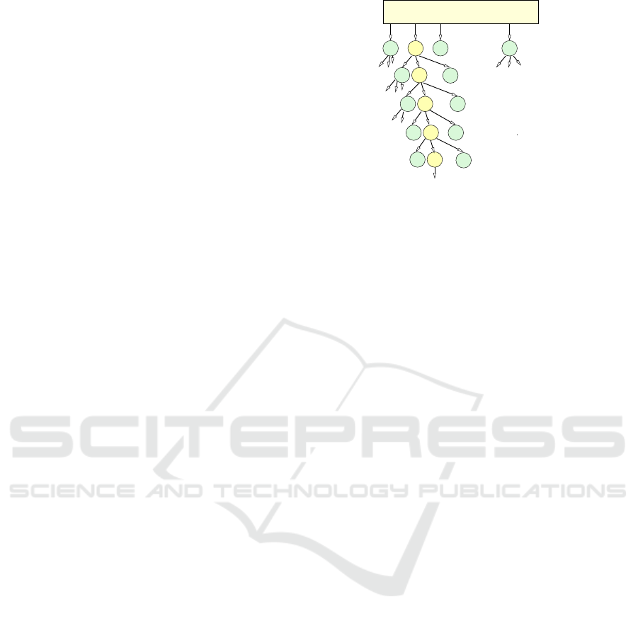
3.2 Variant Generation Process

Figure 1 illustrates the generation of different vari-

ants of numerical solution methods at different lev-

els of the execution pipeline. Starting from a spe-

ciﬁc numerical solution method, different implemen-

tation variants can be generated by different coding of

the main computation loops, e.g., by using different

computation schemes and applying different algorith-

mic optimizations and different program transforma-

tions, including standard transformations such as loop

tiling, loop interchange, loop fusion or loop unrolling.

Each of the different program versions can be

compiled with different compiler options such as op-

tions to enable vectorization, loop optimizations or

alignment. Standard compiler offer a huge number of

different compiler options: the gcc compiler supports

...

implementation

variants

...

number of threads

DVFS settings

compiler options

tolerance values

performance

energy

...

coding timecompile timeruntime

numerical solution method

Figure 1: Illustration of the variant generation process at

different stages of software development and execution, i.e.,

coding time, compile time and runtime. In each level of the

decision tree, a speciﬁc choice of a value for a parameter

can be taken, such that a selection path (depicted as yellow

circles) in the decision tree results. The leaf of a selected

path corresponds to a speciﬁc variant with individual per-

formance and energy data.

more than 200 options and the LLVM compiler has

more than 150 compiler passes (Ashouri et al., 2018).

This large number of options potentially leads to the

possibility to generate a huge number of different exe-

cutables, each with potentially different performance

characteristics. Each of these executables can be ex-

ecuted with different DVFS settings for the cores and

uncores of the execution platform. Moreover, differ-

ent numbers of threads can be employed for the exe-

cution. To control the global error of the approxima-

tion solution, different tolerance values can be used to

control the execution of the numerical method. Over-

all, a potentially huge number of execution variants

results, each with a different performance and energy

behavior.

3.3 Performance of Variants

The execution of an implementation variant V can be

assessed with several performance metrics, such as

the execution time or the energy consumption.

The energy E consumed for the execution of an

implementation variant V during the execution inter-

val [0,t

end

] depends on the given hardware platform

and the power drawing P during the execution time

T = t

end

. The power drawing P may vary during

the execution of the code. Thus, E is expressed as

E =

end

t=0

P(t)dt, assuming that the program is exe-

cuted from time t = 0 to time t = t

end

and that P(t) is

the power drawing at time t.

Several implementation variants can be generated

for a single version of the numerical method. For a

multicore system with p

max

cores, variants for any

Pareto-Optimal Execution of Parallel Applications with Respect to Time and Energy

Table 1: Optimization goals for execution time, energy consumption, and numerical accuracy.

Optimization goals with constraints

execution time energy consumption accuracy

1. minimize no constraint no requirement

2. minimize constraint < E

max

no requirement

3. minimize no constraint requirement < eps

4. no constraint minimize no requirement

5. constraint < T

max

minimize no requirement

6. no constraint minimize requirement < eps

7. no constraint no constraint requirement < eps

8. no constraint constraint < E

max

requirement < eps

9. constraint < T

max

no constraint requirement < eps

10. Pareto-optimization of time and energy no requirement

11. Pareto-optimization of time and energy requirement < eps

12. Pareto optimization of time and energy and accuracy

number of cores between 1 and p

max

can be used. For

DVFS systems with operational frequencies f ranging

between a minimum frequency f

min

and a maximum

frequency f

max

, variants for all available frequencies

can be generated. Starting from f

max

, the maximal

possible scaling factor is s

max

= f

max

/ f

min

. The power

drawing P varies with the number of threads p used

for the execution and the operational frequency f cho-

sen, so that the power P can be expressed as a function

of p and f , i.e., P = P(p, f ), see (Rauber and R

unger,

2012) for more details.

4 ANALYSIS OF PERFORMANCE

DATA

This section is concerned with the performance and

energy data of the calculation of an approximation

solution by a numerical method and the quality of the

approximation solution itself in terms of accuracy. An

analysis of the data provides insight into several ques-

tion with respect to the quality of the solution.

4.1 Performance Optimization Problem

The data concerning the execution time T, the energy

consumption E, the power P as well as the accuracy

Acc in dependence of the operational frequency f ,

the number of threads p and the chosen TOL values

provides a large set of performance data available for

analysis. This data set raises several interesting ques-

tions concerning the behavior that can be investigated

with a suitable data analysis. Especially, the perfor-

mance behavior for computing an approximation be-

havior is an optimization problem to which optimal

or Pareto-optimal solutions are to be found. The opti-

mization problem concerns performance, energy and

accuracy data. The analysis of these performance data

includes the following issues:

• Which relation can be observed between the ex-

ecution time and the energy consumption when

all independent variables f , p,TOL are set to the

same values? Is the relation a linear one or are

there exceptions, e.g., caused by a varying power

consumption?

• How can a best solution be identiﬁed in the two-

dimensional solution space of execution time and

energy consumption? Is there a unique best so-

lution for optimizing both, execution time and

energy consumption, in dependence of p, f and

TOL? Or can a set of of Pareto optimal solutions

be identiﬁed?

• Given an upper bound of the energy consumption

to be invested and an upper bound of the accuracy

(a) Is it possible to ﬁnd suitable values for p, f ,

and T OL so that the related approximation solu-

tion fulﬁlls the constraint? (b) In case that several

feasible solutions are available, which one is the

best or which ones are in the set of Pareto-optimal

solutions?

These questions describe speciﬁc optimization

problems which are of interest. Table 1 summarizes

twelve optimization problems which are possibly in-

teresting to consider. Optimization problems (1) - (3)

minimize the execution time with different constraints

for the energy consumption and the numerical accu-

racy. Problems (4) - (6) minimize the energy con-

sumption with different constraints. Problems (7) -

(9) address minimum requirements for the numeri-

cal accuracy. The three last optimization problems

(10) - (12) describe Pareto-optimal solutions for two

or three objectives, which is formalized in the next

subsection.

SMARTGREENS 2024 - 13th International Conference on Smart Cities and Green ICT Systems

4.2 Deﬁning Pareto-Optimal

Performance of Variants

The problem of ﬁnding an optimal implementation

variant for a numerical solution method can be con-

sidered as a multi-criteria decision problem consider-

ing execution time, energy consumption and numer-

ical accuracy together. For this problem, a decision

space and a criterion space are deﬁned as follows.

Deﬁnition 1. The decision space represents all possi-

ble implementation variants, potentially executed on

a certain number of cores with individual frequency

scaling. The feasible set A is a subset of the decision

space that contains the variants that are available for

the optimization problem.

Deﬁnition 2. The criterion (or objective) space is

the image of the decision space under the objec-

tive function mapping, which are the execution time,

the energy consumption, and the numerical accuracy.

The criterion space for execution time and energy

consumption can be represented by a diagram in

which the x-axis denotes the execution time and the

y-axis denotes the energy consumption.

Each feasible implementation variant V is repre-

sented by a criterion value according to its execution

time and its energy consumption. The image of the

set A under the mappings execution time T : A → R

and energy consumption E : A → R form the feasi-

ble set in the criterion space. The set of feasible

solutions A is built up according to variant generation

process given in Figure 1. The image in the criterion

space is determined by measuring the execution time

and the energy consumption of the different variants

available. The deﬁnition of an efﬁcient implementa-

tion variant in the decision space and the related def-

inition of non-dominated points in the criterion space

are given as follows (Rauber and R

unger, 2019a):

Deﬁnition 3. An implementation variant V is called

efﬁcient (also called Pareto optimal), if there is no

other implementation variant

V such that T (

V ) <

T (V ) and E(

V ) < E(V ). If V is efﬁcient, its entry

(T (V ), E(V )) ∈ R × R in the criterion space is called

non-dominated point. The set of efﬁcient implemen-

tation variants is denoted by A

e f f

. The set of all non-

dominated points is called the non-dominated set.

An implementation variant V

dominates an imple-

mentation variant V

, if T (V

) ≤ T (V

) and E(V

) ≤

E(V

Thus, for the elements in A

e f f

, there exists no al-

ternative that has both a smaller execution time and a

smaller energy consumption. The set of efﬁcient so-

lutions is sometimes also called a Pareto set (Ehrgott,

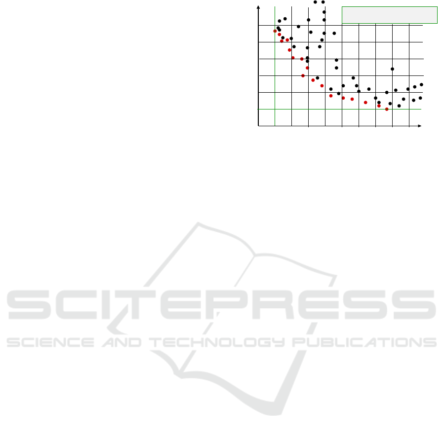
execution time [sec]

energy consumption [J]

Emin

Tmin

Emin: minimum energy consumption

Tmin: minimum execution time

Figure 2: Illustration of the two-dimensional criterion

space with execution time and energy consumption. Each

point represents a different implementation variant. The red

points are the Pareto-optimal points (Rauber and R

unger,

2019a).

2005). In Figure 2, the non-dominated points are de-

picted in red, whereas the black points are points that

are dominated by other points and, therefore, do not

need to be considered further (Rauber and R

unger,

2019a). All red points together represent the Pareto

set. All implementation variants that are not efﬁcient

can be excluded from the search for an optimal so-

lution. For the computation of non-dominated points

and, thus, implementation variants, we use the algo-

rithm in Figure 3.

4.3 Summary of Variant Selection

Figure 3 illustrates the variant selection process for a

parallel application algorithm based on performance

data. In the ﬁrst step (variant generation), a suitable

application algorithm is selected according to the re-

quired accuracy of the solution. The speciﬁc appli-

cation problem to be solved and its characteristics

are taken into consideration for this selection. Usu-

ally, several application algorithms are suitable for the

combination of application problem and the required

accuracy. These different choices lead to different ba-

sic variants to be considered further in the selection

process. Each of these variants potentially leads to

different performance and energy requirements. Each

of the basic variants can be executed with different

parameters of the execution platform, such as differ-

ent numbers of threads and different operational fre-

quencies. Moreover, different implementation vari-

ants can be generated by modifying the loop structure

of the underlying implementation using loop transfor-

mations or by using different compiler options, see

Fig. 3. This potentially leads to a large number of im-

plementation variants that can be executed on the ex-

ecution platform. During the execution, performance

Pareto-Optimal Execution of Parallel Applications with Respect to Time and Energy

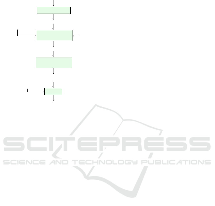
selection

solver variants

execution modes

performance data

specialized

goal

parameters

(DVFS)

optimization

application algorithm

application problem

application variant

application variants

variant generation

cost determination

accuracy measurement

nondominated elements

generation of

Figure 3: Illustration of the variant selection process for a

parallel application algorithm.

data can be collected, including execution times, en-

ergy consumption and numerical accuracy. These

data can then be used construct the time-energy cri-

terion space according to Fig. 2 and to determine the

Pareto set of the variants selected.

The variant selection can be supported by suitable

optimization techniques, see (Gill et al., 1981) for a

detailed treatment. The optimization goal would be

to determine the parameters such that the resulting

energy consumption is minimized. The energy con-

sumption could be captured by a modeling equation

with the expression for T (p, f ) and P(p, f ) written in

such a way that the parameters selected (in this case

the number of threads p and the operational frequency

f ) occur in the expression. Suitable techniques in-

clude constrained methods, where the constraints de-

ﬁne a maximum number of resources that are avail-

able for the execution or a frequency range in which

the frequency value f determined by the optimization

method has to ﬁt.

5 EXPERIMENTAL EVALUATION

The variant selection process is applied to perfor-

mance data of measurements for solving an ODE

test problem with an RK method, see (Rauber and

unger, 2019b) for a detailed description of the RK

solution method. The test ODE results from a spatial

discretization of a two-dimensional time-dependent

partial differential equation describing a reaction-

diffusion (RD) problem of two chemical substances

(Hairer et al., 1993). Discretizations with different

grid sizes N lead to different sizes of the resulting

ODE system.

5.1 Hardware Platforms

For the experimental evaluation, an Intel Broad-

well processor (i7-6950X) has been used. The In-

tel Broadwell i7-6950X CPU has 10 cores on one

socket, running at 3.0 GHz. The TDP is 140 Watt.

Hyper-threading is supported. The memory hierar-

chy includes a 25 MB shared L3 cache, a 256 KB L2

cache and a 32 KB L1 cache per core. The main mem-

ory size is 32 GB. The frequency range supported lies

between 1.2 GHz and 2.9 GHz. Only a discrete set

of frequencies is available: {1.2 GHz, 1.3 GHz, 1.4

GHz, 1.6 GHz, 1.7 GHz, 1.8 GHz, 1.9 GHz, 2.0 GHz,

2.2 GHz, 2.3 GHz, 2.4 GHz, 2.5 GHz, 2.6 GHz, 2.8

GHz, 2.9 GHz }.

The compilation has been performed with the

gcc compiler (Version 7.3.1) using the highest opti-

mization level -O3. The time and energy measure-

ments have been performed using the Running Aver-

age Power Limit (RAPL) interface and sensors of the

Intel architecture (Rotem et al., 2012; Intel, 2011).

RAPL sensors can be accessed by control registers,

known as Model Speciﬁc Registers (MSRs) (Intel,

2011). In particular, the likwid tool-set, especially

the likwid-perfctr tool in Version 4.3.2 (Treibig et al.,

2010) has been used for the experimental evaluation.

The likwid tool-set provides an easy access to the

MSRs. For the experiments with frequency scaling,

likwid-setFrequencies has been used to set the opera-

tional frequency to a ﬁxed value. For the experiments,

only the core frequency has been changed, the uncore

frequency with the memory controller remained un-

changed. The runtime and energy measurements have

been performed with no other user on the system and

no other process except the operating system running

to keep disturbance effects as small as possible.

5.2 Selection of Pareto-Optimal

Variants

In the following, the variant selection process is illus-

trated for the operational frequency used. The vari-

ant selection process is applied to a parallel multi-

threaded implementation version of the DOPRI5 RK

method (Rauber and R

unger, 2019b). As application

problem, the RD ODE using N = 4096 on the Broad-

well processor is considered.

Figure 4 shows the execution time (x-axis) and en-

SMARTGREENS 2024 - 13th International Conference on Smart Cities and Green ICT Systems

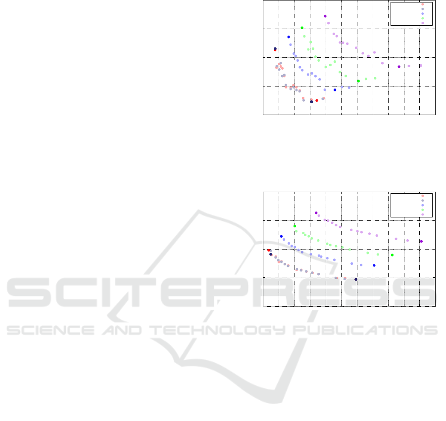
ergy consumption (y-axis) of different implementa-

tion variants executed sequentially on one core of the

Broadwell processor, using different operational fre-

quencies and different tolerance values TOL between

−2

and 10

−6

for the error control and the stepsize

selection. Each dot in the decision space denotes

the value (T (V ),E(V )) for a speciﬁc variant V gen-

erated with a ﬁxed frequency and a predeﬁned toler-

ance value. The diagram shows ﬁve convex curves for

the family of variants that are executed with the same

tolerance value TOL ∈ {10

−3

,10

−4

,10

−5

,10

−6

}. For

each curve, the frequencies decrease from left to right.

The ﬁgure shows that smaller tolerance values

such as 10

−6

lead to larger execution times and larger

energy consumptions that the usage of larger toler-

ance values. This is caused by a higher computational

effort due to the execution of a larger number of time

steps of the ODE method when using a smaller step-

size. The execution times and energy consumptions

for the tolerance values 10

−2

and 10

−3

are quite close

together due to a similar number of time steps.

Figure 4 also shows that the use of the highest op-

eration frequencies leads to the largest energy con-

sumption and the smallest execution time for each of

the different tolerance values. Decreasing the oper-

ational frequency increases the execution time, and

the largest execution time results when using the the

smallest operational frequency. However, the use of

the smallest operational frequency (1.2 GHz) does

not lead to the smallest energy consumption. Instead,

the smallest energy consumption results by using a

slightly higher operational frequency. This frequency

is 1.4 GHz for all tolerance values except 10

−3

, for

which the smallest energy consumption results for 1.3

GHz. Since each of the ﬁve curves represents differ-

ent tolerance values that lead to different numerical

accuracies, the curves have to be considered in isola-

tion. For each of the ﬁve curves, most of the points de-

picted are Pareto points. However, for each of the ﬁve

curves, two important Pareto points can be identiﬁed

that correspond to the smallest energy consumption

and the smallest execution time compared to the other

variants with the same tolerance value. These impor-

tant Pareto points are shown as solid dots in the dia-

gram to distinguish them from the other points, which

are depicted in a lighter color.

Figure 5 shows the same information as Figure

4 using a multithreaded execution with 10 threads.

Again, for each curve the frequencies decrease from

left to right. The important Pareto points are again

shown as solid dots in the diagram. Similar to the

sequential case, the use of smaller tolerance values

leads to larger execution times and larger energy con-

sumptions that the usage of larger tolerance values.

128

256

512

1024

40 60 80 100 120 140 160 180 200 220 240 260

energy [Joule]

execution time [sec]

time/energy for RD ODE p=1 on Broadwell

TOL=10-2

TOL=10-3

TOL=10-4

TOL=10-5

TOL=10-6

Figure 4: Execution time and energy for different frequen-

cies and different tolerance values on Broadwell using a se-

quential execution.

128

256

512

1024

2048

25 30 35 40 45 50 55 60 65 70 75 80

energy [Joule]

execution time [sec]

time/energy for RD ODE p=10 on Broadwell

TOL=10-2

TOL=10-3

TOL=10-4

TOL=10-5

TOL=10-6

Figure 5: Execution time and energy for different frequen-

cies and different tolerance values on Broadwell using a par-

allel execution with 10 threads.

Moreover, the use of the highest operation frequen-

cies leads to the largest energy consumption and the

smallest execution time for each of the different toler-

ance values.

However, there are also several differences be-

tween the diagrams in Figures 4 and 5: For the par-

allel case, the use of the smallest operational fre-

quency always leads to the smallest energy consump-

tion. Moreover, the energy consumption for the paral-

lel execution with 10 threads is much larger than the

energy consumption for a sequential execution. This

is caused by the signiﬁcantly larger power consump-

tion for 10 threads, which cannot be compensated by

a corresponding reduction in execution time.

6 CONCLUSIONS

The execution time and energy consumption for long-

running applications often exhibit a complex interac-

Pareto-Optimal Execution of Parallel Applications with Respect to Time and Energy

tion. There are many inﬂuencing parameter both from

the underlying algorithm and the execution environ-

ment and it is not a priori clear which combination of

parameter values may lead to the best runtime perfor-

mance and the smallest energy consumption.

This article explores the interactions between the

inﬂuencing parameters for a complex example from

numerical analysis and provides a detailed experi-

mental evaluation. The experimental evaluation is

performed for three parameters, one algorithmic pa-

rameter (the tolerance value for the error control) and

one execution parameter (the operational frequency).

The evaluation shows that the interaction between

the runtime performance and the energy consump-

tion is complex and that there is no best combination

that optimizes both the execution time and the energy

consumption. Instead, there are two different Pareto

points, one that minimizes the execution time and one

that minimizes the energy consumption.

REFERENCES

Ahmad, I. and Ranka, S. (2012). Handbook of Energy-

Aware and Green Computing. Chapman & Hall/CRC.

Ashouri, A. H., Killian, W., Cavazos, J., Palermo, G., and

Silvano, C. (2018). A survey on compiler autotun-

ing using machine learning. ACM Comput. Surv.,

51(5):96:1–96:42.

Brown, D. J. and Reams, C. (2010). Toward energy-efﬁcient

computing. Commun. ACM, 53(3):50–58.

Deuﬂhard, P. and Hohmann, A. (2003). Numerical Analysis

in Modern Scientiﬁc Computing, volume 43. Springer.

Ehrgott, M. (2005). Multicriteria Optimization. Springer-

Verlag.

Fard, H. M., Prodan, R., Barrionuevo, J. J. D., and

Fahringer, T. (2012). A multi-objective approach for

workﬂow scheduling in heterogeneous environments.

In 2012 12th IEEE/ACM International Symposium on

Cluster, Cloud and Grid Computing (ccgrid 2012),

pages 300–309.

Freeh, V. W., Lowenthal, D. K., Pan, F., Kappiah, N.,

Springer, R., Rountree, B. L., and Femal, M. E.

(2007). Analyzing the energy-time trade-off in high-

performance computing applications. IEEE Transac-

tions on Parallel and Distributed Systems, 18(6):835–

848.

Gill, P. E., Murray, W., and Wright, M. H. (1981). Practical

optimization. Academic Press Inc. [Harcourt Brace

Jovanovich Publishers], London.

Hairer, E., Nørsett, S., and Wanner, G. (1993). Solving

Ordinary Differential Equations I: Nonstiff Problems.

Springer–Verlag, Berlin.

Intel (2011). Intel 64 and IA-32 Architecture Software De-

veloper’s Manual, System Programming Guide.

Lastovetsky, A. and Manumachu, R. R. (2023). Energy-

efﬁcient parallel computing: Challenges to scaling.

Information, 14(4).

Li, K. (2016). Energy and time constrained task scheduling

on multiprocessor computers with discrete speed lev-

els. Journal of Parallel and Distributed Computing,

95:15–28. Special Issue on Energy Efﬁcient Multi-

Core and Many-Core Systems, Part I.

Li, K. (2018). Scheduling parallel tasks with energy and

time constraints on multiple manycore processors in

a cloud computing environment. Future Generation

Computer Systems, 82:591–605.

Manumachu, R. R., Khaleghzadeh, H., and Lastovetsky,

A. (2023). Acceleration of bi-objective optimization

of data-parallel applications for performance and en-

ergy on heterogeneous hybrid platforms. IEEE Ac-

cess, 11:27226–27245.

Manumachu, R. R. and Lastovetsky, A. (2018). Bi-objective

optimization of data-parallel applications on homoge-

neous multicore clusters for performance and energy.

IEEE Transactions on Computers, 67(2):160–177.

Mezmaz, M., Melab, N., Kessaci, Y., Lee, Y., Talbi, E.-

G., Zomaya, A., and Tuyttens, D. (2011). A paral-

lel bi-objective hybrid metaheuristic for energy-aware

scheduling for cloud computing systems. Journal

of Parallel and Distributed Computing, 71(11):1497–

1508.

OECD (2023). World Energy Outlook 2023. OECD.

Orgerie, A.-C., Assuncao, M. D. d., and Lefevre, L. (2014).

A survey on techniques for improving the energy efﬁ-

ciency of large-scale distributed systems. ACM Com-

put. Surv., 46(4):47:1–47:31.

Rauber, T. and R

unger, G. (2012). Energy-aware Execution

of Fork-Join-based Task Parallelism. In 20th IEEE

International Symposium on Modeling, Analysis, and

Simulation of Computer and Telecommunication Sys-

tems (MASCOTS’12), pages 231–240. IEEE.

Rauber, T. and R

unger, G. (2019a). A Scheduling Selection

Process for Energy-efﬁcient Task Execution on DVFS

Processors. Concurrency and Computation: Practice

and Experience, 31.

Rauber, T. and R

unger, G. (2019b). On the Energy Con-

sumption and Accuracy of Multithreaded Embedded

Runge-Kutta Methods. In Proceedings of the The In-

ternational Conference on High Performance Com-

puting & Simulation (HPCS 2019), volume 15, pages

382–389. IEEE.

Rotem, E., Naveh, A., Ananthakrishnan, A., Rajwan, D.,

and Weissmann, E. (2012). Power-Management Ar-

chitecture of the Intel Microarchitecture Code-Named

Sandy Bridge. IEEE Micro, 32(2):20–27.

Sch

one, R., Ilsche, T., Bielert, M., Gocht, A., and Hack-

enberg, D. (2019). Energy efﬁciency features of the

intel skylake-sp processor and their impact on perfor-

mance. In 2019 International Conference on High

Performance Computing and Simulation (HPCS),

pages 399–406.

Treibig, J., Hager, G., and Wellein, G. (2010). LIKWID:

A Lightweight Performance-Oriented Tool Suite for

x86 Multicore Environments. In 39th International

Conference on Parallel Processing Workshops, ICPP

’10, pages 207–216. IEEE Computer Society.

Zomaya, A. Y. and Lee, Y. C. (2012). Energy Efﬁcient Dis-

tributed Computing Systems. Wiley-IEEE Computer

Society Pr, 1st edition.

SMARTGREENS 2024 - 13th International Conference on Smart Cities and Green ICT Systems