Automatic Identiﬁcation and Classiﬁcation of Map-Matching Anomalies

in Cycling Routes

Carlos Carvalho

1 a

, Mois

es Ramires

2 b

and Rui Jos

1 c

Centro Algoritmi/LASI, University of Minho, Guimar

aes, Portugal

CCG, University of Minho, Guimar

aes, Portugal

Keywords:

OpenStreetMap, Map-Matching, Micro-Mobility, Urban Cycling.

Abstract:

Road network data models are a key element for many cycling services. However, cyclists often ride uncon-

ventional paths that may not be properly represented in those models. This may cause various types of map-

matching anomalies, where the map-matched route does not correspond to the real route. In this work, we

assess a set of classiﬁcation models to automatically detect and classify these map-matching anomalies. Using

OpenStreetMap road network, we generated the map-matched routes for a dataset of 98 cycling GPS traces.

To produce ground-truth data, we visually inspected each result to identify and classify every map-matching

anomaly, and computed several similarity measures between each GPS trace and the respective map-matched

segment. Based on this data, we trained several classiﬁcation models with different feature engineering ap-

proaches to perform binary and multi-class classiﬁcation. The results show that binary classiﬁers can be very

effective in the identiﬁcation of map-matching anomalies. The best model, a XGBoost classiﬁer, obtained

an F1 Score of 0.906 and an accuracy of 0.893, which outperform other methods. However, the multi-class

classiﬁers had lower performance. This ability to automatically detect and classify map-matching anomalies

may help to systematically improve road network models and consequently improve information provided to

cyclists and decision-makers.

1 INTRODUCTION

Urban mobility is a key dimension in sustainabil-

ity strategies. Cities across the world are promot-

ing new mobility policies that foster urban cycling

to help them meet sustainability goals and respond to

net emissions’ mandates (Eguiluz et al., 2022). In-

formation Technology can have a major role in this

transition, empowering cycling mobility with digital

tools that allow citizens to select the best routes based

on their personal preferences, and enabling transit au-

thorities to obtain a rigorous account of cycling activ-

ity and develop data-driven policies. In this context,

Smart Cycling is emerging as a new paradigm based

on shared, real-time, and collaborative application of

data, communications and services, to help best move

people individually, and collectively, across the urban

environment (ECF, 2016).

OpenStreetMap (OSM) is an open-source and col-

https://orcid.org/0000-0001-8052-4178

https://orcid.org/0009-0005-2264-5082

https://orcid.org/0000-0003-3547-2131

laborative project that is commonly used in many cy-

cling information systems and studies (Basiri et al.,

2016; Haklay and Weber, 2008). It represents mul-

tiple types of geographic entities, including the road

network, buildings and administrative limits. Its use

is claimed to be beneﬁcial for reproducibility reasons

and accessibility (Reggiani et al., 2022).

The road network data model, in particular, is a

key enabler for many smart cycling services. It rep-

resents the road network infrastructure and provides

core information for many sorts of mobility services,

including route planning, navigation and vehicle man-

agement, which depend very heavily on the quality of

street network data (Graser et al., 2015).

The OSM road network data model is commonly

used to develop routing engines dedicated for cycling

(Nunes et al., 2021; de Matos et al., 2021; Bergman

and Oksanen, 2016) and to register information about

routes made by cyclists.

Carvalho, C., Ramires, M. and José, R.

Automatic Identiﬁcation and Classiﬁcation of Map-Matching Anomalies in Cycling Routes.

DOI: 10.5220/0012627700003714

Paper published under CC license (CC BY-NC-ND 4.0)

In Proceedings of the 13th International Conference on Smart Cities and Green ICT Systems (SMARTGREENS 2024), pages 17-28

ISBN: 978-989-758-702-3; ISSN: 2184-4968

1.1 Map-Matching Cycling Traces

Map-matching is a key process to analyse cycling ac-

tivity. Its aligns a GPS trace to the most suitable seg-

ments in the road network model. This eliminates the

errors and variations embedded in each trace and pro-

vides an aggregate context to analyse and characterize

trafﬁc.

The efﬁcacy of a map-matching process relies

very strongly on the ability of the road network data

model to offer a very complete representation of the

routes that are effectively being followed by vehicles.

While this is normally a reasonable premise for au-

tomobiles, it is most often not the case with bicy-

cles. Despite the common assumption that bicycles

and other micro-mobility modes will either share the

road with cars or follow some type of cycle path, the

reality of cycling routes is actually much fuzzier. A

realistic cycling journey may include frequent switch-

ing between very heterogeneous roads with very dif-

ferent proﬁles and purposes, such as footpaths, parks

and other unconventional paths that often are not rep-

resented on a road network model (Schweizer et al.,

2016).

Simply creating a road network composed of cy-

cle paths would be simple, but it would not be a realis-

tic solution. Even for the most bicycle-friendly cities,

there is no such thing as a fully segregated bicycle net-

work. Bicycle trips end-up being the result of a multi-

objective optimisation process that comprises the se-

lection of cycling tracks, but also many other types

of roads (Reggiani et al., 2022). Route selection is a

strongly personal choice, and cyclists may combine

very diverse criteria when selecting their preferred

route (Zimmermann et al., 2017). While there may

not be any universally accepted deﬁnition of what a

bike network is, Mekuria et al. (Mekuria et al., 2012),

describe two clearly opposing views on this topic:

from a municipality point of view, a bike network is

deﬁned as the set of links that cyclists are permitted

to use, whereas, from a user perspective a bike net-

work is the set of streets and paths that do not exceed

people’s tolerance for trafﬁc stress.

The main consequence, therefore, is that when

we consider cycling, map-matching processes will of-

ten fail, not necessarily because of their algorithms,

but because the route that is being taken is not prop-

erly represented in the OSM road network model.

This can have a major impact in the quality of Cy-

cling Analytics Systems and the subsequent analy-

sis of travel behaviour (Berjisian and Bigazzi, 2023).

Mismatched routes could, for example, lead to erro-

neous data on walking and cycling volumes or incor-

rect inferences on travelling preferences. Detecting

and avoiding these anomalies is therefore essential

to ensure the quality of the insights being offered to

decision-makers and cyclists. However, there is still

limited research on detecting and understanding these

map-matching mismatches (Qu et al., 2023), and

the process of detecting the map-matching anomalies

still mainly resorts to visual inspection and reasoning

(Dey et al., 2022).

1.2 Objectives

In this study, we assess and propose a machine

learning approach for detecting and classifying map-

matching anomalies resulting from map-matching cy-

cling traces to OSM. Given a particular GPS trace rep-

resenting a route effectively taken by a cyclist, we de-

ﬁne an anomaly as a portion of that trace for which

map-matching either fails to produce a match or pro-

duces a match to a segment that is not representative

of the GPS trace.

The research objectives are as follows:

• Deﬁne and assess a machine learning approach to

detect relevant discrepancies between a GPS trace

and the GPS route produced by a map-matching

algorithm.

• Deﬁne and assess a machine learning approach to

classify those anomalies according to their main

cause.

The main contribution of this work is a novel ap-

proach to detect and classify map-matching anoma-

lies using machine learning. This new approach

will open the door for the large scale assessment of

the representativeness of road network data models

across multiple cities, and subsequently inform pro-

cesses for improving those models or even the cycling

network itself.

2 RELATED WORK

Previous research has studied the topic of how accu-

rately OSM represents the cycling network infrastruc-

ture and how well it supports cycling-related services.

In this section, we explore three different perspec-

tives, namely OSM quality, map-matching and iden-

tiﬁcation of map-matching anomalies.

2.1 OSM Quality for Cycling

A study by Hochmair et al. (Hochmair et al., 2015)

identiﬁes two main types of errors, namely omission

and commission errors. Omission errors occur when

a cycle lane is not represented in the OSM database or

SMARTGREENS 2024 - 13th International Conference on Smart Cities and Green ICT Systems

does not include proper cycling tags. Commission er-

rors occur when a non-existing road is represented in

the OSM database, either by incorrect geometry deﬁ-

nition or by incorrect use of cycling tags.

To assess OSM completeness, previous studies

(Ferster et al., 2020; Hochmair et al., 2015) com-

pared the OSM road network database against ref-

erence data obtained from municipalities, planning

agencies or from Google Maps. This assessment is

often achieved by comparing the total length of the

road network databases under analysis, either glob-

ally or separately for each road category.

In a study comparing OSM road network with

data for US and European cities, Hochmair et al.

(Hochmair et al., 2015) found that OSM data has rel-

atively good quality, and particularly high quality for

designated lanes. In another study, comparing OSM

data with reference data for six Canadian cities, Fer-

ster et al. found that OSM has very high concordance

in two cities and moderately high concordance in the

other four (Ferster et al., 2020). In some cases, OSM

data was even more detailed than reference datasets.In

their study, on-street bicycle lanes were the most con-

sistent, while cycle tracks and local street bikeways

were the least consistent. As the OSM database is de-

pendant of crowd-sourced contributions, a key chal-

lenge is to achieve consistent OSM tagging for differ-

ent bicycle infrastructures types, as people from dif-

ferent places can have different interpretations of the

same tag or the same interpretation for different tags

(Ferster et al., 2020).

With a different perspective, Wasserman et al.

evaluated the potential of OSM to assess the level of

trafﬁc stress (LTS) (Wasserman et al., 2019), a promi-

nent metric to measure the facilities attractiveness for

cycling. The authors compared OSM-derived LTS

predictions with ground-truth LTS scores, and found

high concordance, with 89.9% of the length of the net-

work being correctly identiﬁed as either high or low

stress. However, some street typologies and urban

contexts are more prone to errors. It includes areas

that might be under-represented in tag completeness,

such as suburban or rural locations, and in denser ar-

eas, where street typologies might be more complex

and potentially misrepresented in OSM . Graser et al.

(Graser et al., 2015) analysed the quality of OSM road

network for performing vehicle routing. By compar-

ing OSM with the Austrian reference graph, the au-

thors conclude that there is a close alignment between

the one-way street and turn restriction information.

These studies suggest that OSM can effectively

represent cycling activities and be the foundation for

many cycling related studies. OSM has generally

good quality, but the level of completeness varies de-

pending on the region and the road category. The

problems identiﬁed, such as missing roads and incon-

sistent tagging, reduce the quality of routing and map-

matching processes, making it essential to have tools

and methodologies that can identify them and correct

them in a systematic way.

2.2 Map-Matching Algorithms

Map-matching algorithms are a key element for trans-

port modelling. Their purpose is to ﬁnd the most suit-

able sequence of road network edges on which a ve-

hicle has travelled based on a GPS trace and a road

network model (Yang and Gid

ofalvi, 2018). How-

ever, applying map-matching on bicycle trips is par-

ticularly challenging as cyclists often use roads which

may not be represented by the road network model,

such as parks or dirty roads (Berjisian and Bigazzi,

2023; Schweizer et al., 2016). Additionally, the road

network data may be incomplete, thus map-matching

algorithms need to be tolerant to this lack of informa-

tion (Sultan et al., 2017).

The built environment has also a strong inﬂu-

ence on the performance of map-matching algorithms

(Trogh et al., 2022). In areas with a sparser road net-

work (e.g. countryside), the chances of map-matching

anomalies are much smaller than in dense urban areas

where multiple parallel roads may exist and tall build-

ings may lead to noisy GPS signals. This makes the

process of map-matching urban cycling routes even

more challenging.

Several studies tried to address these limita-

tions by proposing new map-matching algorithms.

Bergman and Oksanen (Bergman and Oksanen, 2016)

proposed a method based on Hidden Markov Model

(HMM), which favoured bikeways extracted from

Open Street Map (OSM) to perform map-matching.

Schweizer et al. (Schweizer et al., 2016) proposed a

buffer-based map-matching algorithm that maximizes

the likelihood that a route is identical to the real route

from where the GPS trace has been sampled. They

create buffers that encircle edges to determine the

probability of ﬁnding GPS points near edges. It uses

network attributes to estimate the route in case of in-

complete GPS data and can identify if cyclists used

a reserved bikeway, where available. Trogh et al.

(Trogh et al., 2022) proposed a map-matching algo-

rithm that supports trajectories on foot, by bike, and

by motorized vehicles. It combines Markovian be-

haviour and the shortest path aspect while consider-

ing the type and direction of road segments, one-way

trafﬁc, maximum speed, and driving behaviour. De-

pending on the transportation mode, some roads are

discarded from the grid based on their tags. For exam-

Automatic Identiﬁcation and Classiﬁcation of Map-Matching Anomalies in Cycling Routes

ple, if the trace is labelled as on bike, highway roads

are excluded.

Other approaches acknowledge the incomplete-

ness of the road network and use the GPS trace to ex-

tract new road information. Sasaki et al. (Sasaki et al.,

2019) proposed an algorithm to interpolate missing

road segments by using vehicle trajectories based on

map-matching and clustering techniques.

Behr et al. (Behr et al., 2021) proposed an ap-

proach that allows map-matching of trajectories that

possibly contain on- and off-road sections, as cy-

clists and pedestrians can go through roads omitted

in the road network and through open areas, such as

parks. They called these semi-restricted trajectories.

They extend the road network by triangulating all

open spaces and add tessellation edges to the graph.

The approach is based on a state-transition model,

and consider each GPS point as possible (additional)

matching candidate. The unmatched candidates are

added as nodes in road network graph if no path in

the road network is similar to the trajectory.

In other study, Murphy et al. (Murphy et al., 2019)

proposed a map-matching algorithm for on and off-

road tracking. For this, the algorithm switch between

two modes as necessary: It uses standard HMM (Hid-

den Markov Model) to perform on-road vehicle map-

matching, and uses a closed form Kalman Filter for

free-space tracking. Off-road trajectory portions are

generated to be used as fall-back when the road can-

not accommodate the observed vehicle motion. The

sIMM (semi-interacting multiple model) ﬁlter is used

to calculate model probabilities at each step. In cases

where it detects map errors or omissions, the algo-

rithm tries to correct them.

2.3 Automated Identiﬁcation of

Map-Matching Anomalies

The common way to identify map-matching anoma-

lies is through visual inspection (Dey et al., 2022).

This is a tedious and time consuming task, that is only

viable for small scale studies.

Dey et al. (Dey et al., 2022) proposed a method

to identify map-matching anomalies with two distinct

phases. In the ﬁrst phase, using unsupervised learn-

ing, they classify each GNSS point as good or bad

based on its orthogonal distance to the map-matched

segment and the estimated GNSS error obtained from

a Gaussian mixture model. Then, the map-matched

segments are voted as good or bad, based on the ma-

jority of points associated with them. In the second

stage, they use the ”edit distance” to detect unrealistic

behaviour based on trajectory reversal. However, they

assume that the road network is complete and do not

consider the speciﬁc behaviour of cycling. Unlike au-

tomobiles, cyclists can easily reverse their trajectory,

thus making this method unsuited for cycling routes.

In a another study, Berjisian and Bigazzi

(Berjisian and Bigazzi, 2023) evaluated several open-

source map-matching algorithms for active travel.

They concluded that pgMapMatch is the best algo-

rithm, however, it is not designed speciﬁcally for cy-

cling. They also proposed an error detection measure

to ﬂag potential map-matching anomalies requiring

visual inspection. Their method is based on the sim-

ilarity between the GPS trace and the map-matched

route. In our study, we re-purpose some of the sim-

ilarity measures, but the novelty is their use as in-

put data for a supervised machine learning process

that can automatically detect and classify the map-

matching anomalies.

3 METHODOLOGY

The methodology for this study is based on a se-

quence of steps aiming to collect the necessary data

(GPS traces and road network data models), map-

matching the routes, analysing the results of the

map-matching process and training a machine learn-

ing model to identify and characterize map-matching

anomalies.

3.1 Data Acquisition and Preparation

To guarantee diversity and authenticity, we acquired

real routes from four very distinct cities, regarding

their size, cycling culture, and mobility policies, more

speciﬁcally: Braga (Portugal), Seville (Spain), Paris

(France) and Amsterdam (Netherlands). Using the

wikiloc

website, we searched for cycling routes in

the selected areas and downloaded a set of at least 20

GPS traces of routes that had been effectively made

by cyclists in each of those cities, resulting in a total

of 98 GPS traces with a total length of 894 Km.

To improve the granularity of the analysis and

fully understand the behaviour of the map-matching

process, we divided these traces in slices of approx-

imately 1000 meters, depending on the distance be-

tween consecutive GPS points. The last slice of

each GPS trace was composed of the remaining GPS

points, and would thus be smaller than 1000 meters.

This resulted in 935 trace slices.

https://www.wikiloc.com/

SMARTGREENS 2024 - 13th International Conference on Smart Cities and Green ICT Systems

3.2 Road Network Data

For each of the selected cities, we created a database

with the respective OSM road network model. We

started by obtaining the road network data, using the

geofabrik

website. Secondly, we used the osmium

tool to select the data corresponding to the main ur-

ban area. Then we applied the osm2po

tool to con-

vert the selected road network model into a routable

model. For this conversion, we considered car, pedes-

trian and cyclist roads. Finally, we created an instance

of a PostgreSQL

database with PostGIS extension

and imported the topology data using the psql

tool.

3.3 Map-Matching

In this study, our focus is not on the quality or any par-

ticular properties of map-matching algorithms. We

are only concerned about the discrepancies between

the road network model and the real routes used by

cyclists. To reduce any effects of the algorithm selec-

tion on the results of our study, we opted for pgMap-

Match (Millard-Ball et al., 2019). This is a widely

used algorithm, which has been classiﬁed as the best-

performing algorithm in a study by Berjisian and

Bigazzi (Berjisian and Bigazzi, 2023) and seemed ac-

ceptable as a representative example of the current

state of art in map-matching algorithms.

We thus used pgMapMatch to perform a map-

matching operation in each of the slices obtained in

the previous step. For each city, we started by con-

ﬁguring the pgMapMatch

tool to use the respective

database instance as the source data for map-matching

processes. Finally, we map-matched each GPS trace

slice into the OSM road network model and built the

resulting geometry.

3.4 Ground-Truth Data

To obtain ground-truth data, we visually inspected the

map-matching results to identify and categorize every

anomaly. For each slice, we generated a map visu-

alization representing the road network, the original

GPS trace slice and the map-matched route. We then

analysed each of the 935 visualizations to identify any

anomalous situations. In this context, an anomaly was

a case where it was obvious from visual inspection

https://www.geofabrik.de

https://osmcode.org/osmium-tool/

https://osm2po.de

https://www.postgresql.org

https://www.postgresql.org/docs/current/app-

psql.html

https://github.com/amillb/pgMapMatch

that the map-matched route was not the best option

for representing the route taken by the cyclist. Ex-

cept for some concurrent roads, this is one of those

problems where Human reasoning can be very effec-

tive at disambiguating anomaly situations by consid-

ering background knowledge about cycling and land

usage in the area represented by the map. The catego-

rization was based on the type of apparent source of

the anomaly. In some cases, assessing the cause for

the anomaly required the inspection of the OSM road

network data to get details about road types and tags.

3.5 Generation of Similarity Measures

At this stage, we computed several similarity mea-

sures for each GPS trace slice and the corresponding

map-matched route. They are all based on literature

and some of them were also used by Berjisian and

Bigazzi (Berjisian and Bigazzi, 2023).

GPS Trace Slice Length (TL). The total length of

the GPS trace slice.

Map-Matched Route Length (ML). The total

length of the map-matched route.

Length Index (LI). The ratio between the length

of a GPS trace slice and the respective map-matched

route (Schweizer et al., 2016). In optimal scenarios,

this value would be close to 1.

Average Distance (AD). The average value of the

distances between each GPS trace and the respective

map-matched route. This metric uses the distance

between each point in the GPS trace and the near-

est point in the map-matched route. The order of the

points is not considered (Schweizer et al., 2016).

Average Distance Error per Record (ADE). The

average value of the distances between each GPS

trace and the map-matched route, as proposed by

Berjisian and Bigazzi (Berjisian and Bigazzi, 2023).

This approach considers the distance to two possible

map-matched route segments, particularly the one as-

signed to the last GPS point and the following. The

smaller distance is used. However, if the cumulative

distance between the ﬁrst GPS point assigned to the

ﬁrst segment and the current GPS point is longer than

the length of the ﬁrst map-matched segment, the dis-

tance to the second is always used, and this process

recommences.

Automatic Identiﬁcation and Classiﬁcation of Map-Matching Anomalies in Cycling Routes

Discrete Fr

echet Distance (FD). The Fr

echet Dis-

tance assesses the similarities between two geome-

tries. It can be explained as: A man walks a dog with

a leash. They walk on two curves independently with

varying speeds. The Fr

echet distance is the minimum

leash length required to traverse both curves (Eiter

and Mannila, 1994). The higher the Fr

echet distance

is, the less similar both curves are. There are multiple

variants of this metric. In the weak Frechet variant,

one or both ”entities” can walk backwards. We use

the strong Fr

echet variant, where only movement for-

ward is allowed. The discrete variant is an approxi-

mation for polygonal curves.

Dynamic Time Warping (DTW). Dynamic Time

Warping (DTW) is used in many areas to measure

the similarity or the distance between two sequences

(Toohey and Duckham, 2015). In the context of our

study, the sequences are composed of long/lat pairs,

one represents the GPS trace and the other the map-

matched route. The distance between each pair of

points is computed with the haversine formula.

Alignment (A). The alignment metric, as proposed

by Berjisian and Bigazzi (Berjisian and Bigazzi,

2023), describes the average difference between the

bearings of the GPS trace and the corresponding map-

matched route over each 5 consecutive GPS points.

To obtain the start point of the corresponding map-

matched route segment, the ﬁrst GPS point of the in-

terval is projected into the map-matched route. The

last point of the map-matched route segment is ob-

tained by walking on the map-matched route a dis-

tance equal to the cumulative distance between the

GPS points considered.

3.6 Classiﬁcation Models

Supervised machine learning classiﬁcation aims to

categorize data or predict outcomes based on prior

labelled information (Singh et al., 2016). It is used

in many data science problems and comprehends two

phases. First, the classiﬁer is trained using a training

dataset. Then, the performance of the resulting model

is evaluated against a labelled test data.

In the context of our work, we started by train-

ing a set of binary classiﬁers using the similarity mea-

sures as features and the ground-truth data as labels.

The objective of these models was to detect the map-

matching anomalies.

Later, using the same dataset, we trained and

tested several multi-class classiﬁers to identify the

probable cause of these anomalies.

In each stage, we tested different feature engi-

neering approaches, and conducted hyperparameteri-

zation with cross validation to improve the conﬁdence

on the results.

We considered several metrics for assessing the

performance of the classiﬁcation models. For the bi-

nary classiﬁcation models, we computed the accu-

racy, precision, recall, and F1 Score (Iwendi et al.,

2020; Gyawali and Qian, 2019), and for the multi-

class models, we considered accuracy and macro pre-

cision, recall, and F1 Score (Takahashi et al., 2022).

These metrics are well known, and used frequently in

machine learning related studies.

4 RESULTS

In this section, we describe the results of our study.

We start by describing and analysing the results ob-

tained by applying the map-matching algorithm into

selected GPS traces. After, we proceed to describe

the training and application of the binary classiﬁers.

Then, we present the results of performing multi-class

classiﬁcation. Finally, we assess the Berjisian and

Bigazzi method to detect map-matching anomalies

(Berjisian and Bigazzi, 2023) and compare its perfor-

mance against our binary classiﬁcation.

4.1 Analysis of the Map-Matching

Process

The ﬁrst part of this study involved collecting GPS

traces representing bicycle activity, slice them into

smaller portions, map-matching the resulting slices

into OSM and performing visual inspection of the re-

sults to produce ground truth data. We used the GPS

trace slice as our unit of analysis.

The visual inspection of the routes produced by

the map-matching algorithm, allowed us to identify

and classify the map-matching anomalies. Table 1 de-

scribe the overall results and ﬁgure 1 shows 6 exam-

ples of common map-matching anomalies.

Out of the 935 slices analysed, 417 cases (44,6%)

were entirely map-matched with success. The re-

maining 518 slices (55,4%) had at least a small por-

tion with a faulty map-matched situation. In some

cases, the map-matching process failed at several por-

tions across the slice. In 45 of those slices (4,8%),

the map-matching even failed due to different reasons.

As result, these cases were assigned to multiple cate-

gories.

Comparing the map-matching results for each

city, we observe that the success rate varied slightly.

Amsterdam had the lowest success rate with 39,8%,

SMARTGREENS 2024 - 13th International Conference on Smart Cities and Green ICT Systems

Table 1: General stats: Map-matching anomalies.

Braga Amsterdam Paris Sevilha Total

GPS Traces 24 22 20 32 98

Total Length (Km) 213 179 96 406 894

GPS Trace Slices 226 191 98 420 935

% of Slices Without Error 44,7 39,8 42,9 47,1 44,6

% of Slices With At Least 1 Error 55,3 60,2 57,1 52,9 55,4

% of Slices Assigned to One Error Category 50,9 59,2 45,9 47,6 50,6

% of Slices Assigned to Multiple Error Categories 4,4 1,0 11,2 5,2 4,8

Figure 1: Examples of common map-matching anomalies:

1- Competing roads; 2- GPS error; 3- Missing Segment; 4-

One-way; 5- Map-matching; 6- Open Area.

while Seville has the highest one with 47,1%. This

can be somewhat explained by the source of the

anomalies. In Amsterdam, the majority of these

anomalies were caused by ”one-way” travel against

trafﬁc direction, which the map-matching algorithm

does not consider, even in cases where the cyclist used

cycleways.

The manual classiﬁcation of the anomalies is rep-

resented in Table 2, which summaries the occurrences

per category in each city. Since the total number of

slices varies substantially across cities, we computed

two ratios. The ﬁrst, Rt, shows the ratio of occur-

rences of each category per GPS trace slice. The sec-

ond, Re, shows the ratio of occurrences of each cate-

gory per anomaly. Since one map-matching anomaly

can be assigned with one or more categories, the sum

of Re can be higher than 100%. As we can see, de-

spite similar map-matching success rates, the main

source of error varies substantially across city.

The three main sources of anomalies were di-

rectly related to the road network, namely one-way,

competing-roads, and missing segments. This is

in line with the results from Berjisian and Bigazzi

(Berjisian and Bigazzi, 2023). They also point out

that the most common sources of error were cyclists

travelling in the wrong direction on a one-way street,

travelling on missing links, and traces being map-

matched to a parallel street.

The map-matching algorithm itself led to 78

anomalies. In those cases the algorithm wrongly re-

turned the last portion of the map-matched segment

duplicated. This would mean that the cyclist inverted

his direction of travel. However, by visually inspect-

ing the results, we could observe that it was not the

case.

Bad GPS trace quality led to 44 map-matching

anomalies. In some cases, strong interferences on the

GPS signals led the measurements to be recorded as

being above buildings or rivers. In other cases, the

GPS traces had a very low sampling rate or had long

intervals without recordings. These situations jeopar-

dised the map-matching process.

Finally, we tagged 5 cases as ”unknown” as we

could not properly identify their main cause.

4.2 Binary Classiﬁcation for Anomaly

Detection

After performing the ground-truth analysis, we com-

puted the similarity measures between each GPS trace

slice and the corresponding map-matched route. We

then developed a Python script to train and test binary

classiﬁcation models, using sklearn

library. We con-

sidered 8 different classiﬁers, namely: Logistic Re-

gression, SVC, K-Neighbors (KNN), Decision Tree,

Random Forest, Gaussian Naive Bayes, XGBoost and

Adaboost.

We used 75% of the labelled data as the training

dataset and the remaining 25% to evaluate their per-

formance. The data were shufﬂed randomly before

splitting. We performed Random Search with 4-fold

cross validation to ﬁnd the best hyperparameters for

each classiﬁer and to increase conﬁdence on the re-

sults.

https://scikit-learn.org/stable/

Automatic Identiﬁcation and Classiﬁcation of Map-Matching Anomalies in Cycling Routes

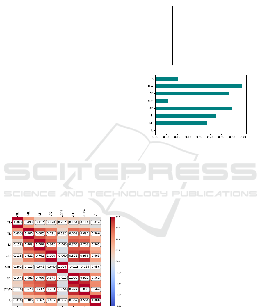
Table 2: Category occurrences per city.

Dataset Braga Amsterdam Paris Sevilha Total

Category Cnt Rt Re Cnt Rt Re Cnt Rt Re Cnt Rt Re Cnt Rt Re

One-Way 53 23,5 42,4 71 37,2 61,7 30 30,6 53,6 52 12,4 23,4 206 22,0 39,8

Competing Road 9 4,0 7,2 21 11,0 18,3 20 20,4 35,7 72 17,1 32,4 122 13,0 23,6

Missing Segment 39 17,3 31,2 2 1,0 1,7 3 3,1 5,4 54 12,9 24,3 98 10,5 18,9

Map-Matching 24 10,6 19,2 2 1,0 1,7 3 3,1 5,4 49 11,7 22,1 78 8,3 15,1

GPS 2 0,9 1,6 18 9,4 15,7 11 11,2 19,6 13 3,1 5,9 44 4,7 8,5

Open-Area 5 2,2 4 0 0 0 0 0 0 2 0,5 0,9 7 0,7 1,4

Uknown 2 0,9 1,6 2 1,0 1,7 0 0 0 1 0,2 0,5 5 0,5 1,0

Circular Street 0 0 0 0 0 0 0 0 0 1 0,2 0,5 1 0,1 0,2

Complex Crossing 1 0,4 0,8 0 0 0 0 0 0 0 0 0 1 0,1 0,2

No Bicycle 0 0 0 0 0 0 1 1,0 1,8 0 0 0 1 0,1 0,2

We used four different feature engineering ap-

proaches namely ANOVA, Principal Component

Analysis (PCA), Mutual Information and the Spear-

man correlation between features (Khalid et al.,

2014). For each approach we also tested with stan-

dardised valued (STD). Depending on the approach,

we used different set of features:

• ”None”. We used every feature available.

• ”Corr”. Based on the Spearman correlation be-

tween features shown ﬁgure 2, we removed highly

correlated features, using only the TL, ADE,

DTW, and A.

• ”Info-Gain”. We considered the features with

most dependency with the result, namely DTW,

FD, AD, and LI. The results of mutual informa-

tion analysis is shown in ﬁgure 3.

• ”PCA”. We considered 4 components.

• ”ANOVA”. We used 6 features.

Figure 2: Spearman Correlation between features.

Regarding the dataset, out of the 935 map-

matching requests, 518 (55%) had anomalous results,

showing that our dataset is balanced for the error iden-

tiﬁcation phase. Table 3 shows a summary of the

results for the binary models, ordered by accuracy

Figure 3: Information Gain.

Table 3: Binary Classiﬁcation Results - Short Version.

ID Model Version Prec. Recall F1 Acc.

1 XGB ANOVA 0,883 0,931 0,906 0,893

2 XGB ANOVA-STD 0,883 0,931 0,906 0,893

3 DT Info-Gain 0,888 0,915 0,902 0,889

4 KNN Corr 0,876 0,923 0,899 0,885

5 KNN None 0,876 0,923 0,899 0,885

6 KNN ANOVA 0,887 0,908 0,897 0,885

7 XGB Corr 0,887 0,908 0,897 0,885

... ... ... ... ... ... ...

56 SVC None 0,573 1,000 0,728 0,585

score. ”Version” column correspond to the feature se-

lection algorithm.

Results show that the performance of the models

varied considerably, depending on the classiﬁer algo-

rithm and the feature engineering method used. Some

models had a very low performance, with accuracy

below 0.6.

However, other models had a very good perfor-

mance, with accuracy close to 0.89. The best per-

forming model was a trained Extreme Gradient Boost

(XGB) with ANOVA feature selection. It was also the

model with best F1 Score, slightly above 0.9. Addi-

tionally, there were several other models which were

very similar in performance, including Decision Tree,

Adaboost and Logistic regression.

This results show that with binary classiﬁca-

tion models it is possible to identify map-matching

anomalies with very good conﬁdence.

SMARTGREENS 2024 - 13th International Conference on Smart Cities and Green ICT Systems

4.3 Multi-Class Classiﬁcation for

Anomaly Classiﬁcation

In the second phase of our work, we trained a slightly

different set of multi-class classiﬁers. This included

Naive Bayes (NB), Random Forest (RF), Logistic Re-

gression (RF), Decision Tree (DT), KNN, and SVC.

We used the same ground-truth data and similar-

ity measures. However, we excluded the occurrences

tagged with multiple categories and the categories

with less than 20 occurrences, due to low represen-

tativeness.

We used 75% of the dataset for training, and the

remaining 25% for testing. We conducted Random

Search of the hyperparameters with 4-fold cross val-

idation. We tested these models using different types

of feature engineering, namely PCA, mutual informa-

tion, Spearman correlation, and ANOVA. In some it-

eration, we applied SMOTE preprocessing algorithm

(Fernandez et al., 2018) to balance the error cate-

gories. In the iterations tagged as ”-SMT-U”, we as-

sessed how the performance of these models varied

if we performed SMOTE to oversampling the minor-

ity categories up to 100 entries and downsampling the

”OK” category to just 200 occurrences. Table 4 shows

the initial training dataset, and the training dataset af-

ter performing feature engineering for this iteration.

Table 4: Train Dataset for the iteration: ”-SMT-U”.

Train Dataset Test Dataset

Category Before After (SMT-U) Count

OK 309 200 108

Missing Segment 58 100 20

Competing Road 72 100 29

Map Matching 59 100 8

One-way 128 128 47

GPS 31 100 7

Total 657 728 219

Table 5 presents the performance of the top trained

models, sorted by accuracy.

Table 5: Multi-class classiﬁcation Results - Short Version.

ID Model Version Prec. Recall F1 Acc.

1 RF None 0,63 0,57 0,59 0,71

2 RF Info-Gain 0,57 0,54 0,53 0,68

3 RF ANOVA 0,59 0,53 0,54 0,68

4 RF Corr 0,47 0,41 0,41 0,68

5 DT ANOVA 0,54 0,51 0,50 0,68

6 LR PCA 0,45 0,40 0,39 0,68

... ... ... ... ... ... ...

90 LR Info-Gain-SMOTE 0,04 0,26 0,05 0,06

In general, the results indicate that the perfor-

mance of multi-class classiﬁcation models is bad. The

majority of these models can easily identify that an

anomaly has occurred. However, they often fail to

identify their probable cause.

Figure 4 shows the confusion matrix for the best

performing model. We can observe that, out of the

104 cases predicted as ”OK”, 92 were predicted cor-

rectly. This was from a total of 108 true ”OK” cases.

We can also observe that many of the map-matching

occurrences categories were wrongly predicted. As

example, the majority of ”missing-segment” cases

were predicted as ”one-way”. Another example is

that 12 out of 47 ”one-way” cases were predicted with

other labels.

Figure 4: Confusion matrix for the RF model with no fea-

ture engineering.

In a real-world application, this multi-class clas-

siﬁcation models could complement the identiﬁcation

made by the binary. Spite bad performance, their out-

puts can act as suggestions about the probable cause

of failure. These suggestions are valuable to people

responsible for manually inspecting the results, ﬁnd-

ing where the road network model is incomplete and

making the right adjustments.

4.4 Error Indicator Method Assessment

The ﬁnal part of our work consisted of assessing the

quality of Error Indicator (EI) to detect map-matching

anomalies and comparing its performance with the bi-

nary classiﬁcation models. The EI method is one of

the few methods that does not use ground-truth data to

detect map-matching anomalies. It was proposed by

Berjisian and Bigazzi (Berjisian and Bigazzi, 2023),

and consisted of equation 1, as follows:

= 0.39LI

′

+ 0.94ADE

′

+ 0.67A

′

+0.96DTW

′

+ 0.74FD

′

(1)

This expression uses normalized values for each

component, corresponding to the similarity measures

Automatic Identiﬁcation and Classiﬁcation of Map-Matching Anomalies in Cycling Routes

deﬁned in section 3.5. The LI component was ob-

tained by computing the absolute value of the Length

Index - 1, as map-matched routes shorter than the

GPS trace (LI <1) would contribute negatively to the

EI result. It is important to state that the normalization

process was made based on the range of values for

each dataset separately. In their work, entries with EI

values greater than 0.5 were ﬂagged for visual inspec-

tion as potentially unreliable results. Table 6 shows

the results of applying this method to our datasets.

Table 6: Error Indicator Performance.

Braga Amsterdam Paris Seville Total

Accuracy 0,77 0,63 0,77 0,55 0,64

Precision 0,81 0,79 0,72 0,84 0,79

Recall 0,76 0,52 0,96 0,19 0,48

F1 Score 0,78 0,63 0,82 0,31 0,6

In total, out of the 518 anomalies, the EI correctly

ﬂagged 251 and missed 267. This is an overall re-

call value of 0.48. Additionally, 68 cases without

anomaly were wrongly ﬂagged for visual inspection.

This makes an overall precision value of 0.79, mean-

ing that, on average, 1 in every 5 cases was ﬂagged

incorrectly for visual assessment.

Comparing the results for each dataset, we ob-

serve that they varied substantially. For smaller

datasets, EI had a good sensibility to detect anoma-

lies, but created more false positives. On the contrary,

with larger datasets, precision increased, but the sen-

sitivity to detect anomalies experienced a signiﬁcant

decline.

This was due to the occurrence of outliers with

bigger discrepancies between the GPS trace and the

map-matching result, as their similarity measures

tend to have a strong negative inﬂuence during the

normalization phase. This impact reduces the sensi-

bility of EI to detect smaller anomalies.

Additionally, the performance of this method var-

ied across categories. Table 7 shows the recall values

for the ﬁve most common categories. These can be

interpreted as the number of occurrences of a given

category that were ﬂagged for visual inspection since

EI only performs detection and does not classify the

occurrences.

We can observe that EI hardly detected the ”Com-

peting Road” occurrences. For this type of anoma-

lies, EI had a recall value equal or below 0.13 on 3

datasets, with exception for the ”Paris” dataset.

This was caused by the existence of outliers in

bigger datasets. In ”competing road” anomalies,

the differences between the GPS trace and the map-

matching is very subtle, and their similarity measures

tend to be approximate to the similarity measures

from cases where map-matching was correct. As the

values were normalized, the occurrence of outliers

hide those differences, and pass undetected by the EI

method. Even for anomalies that are characterised

by strong differences between the GPS trace and the

map-matching result, such as one-way or missing seg-

ments, EI obtained a recall value of 0.17 and 0.38 for

the Seville dataset.

4.4.1 Comparison Between EI and ML

Approach

If we compare the performance of both approaches,

we observe that binary classiﬁcation models outper-

form EI method by a large margin. The top binary

classiﬁcation model obtained an accuracy of 0.893

and F1 score of 0,906, while the EI method obtained,

on average, an accuracy of 0,64 and a F1 Score of 0,6.

Additionally, the EI method does not give hints about

the root cause of the anomaly. Despite the low perfor-

mance of the multi-class models, these hints can be

very useful for people responsible of correcting OSM

data.

Another advantage of our approach is the ability

to detect anomalies in real-time. It does not require

the normalization of the value prior to the veriﬁcation,

while EI requires the normalization of its measures

before obtaining the ﬁnal value. This makes the ML

approach better suited for real-world scenarios, where

there are many routes being recorded every second.

5 CONCLUSIONS

Detecting the gaps between real cycling routes and

how they are matched to the existing road network

data model is an essential ﬁrst step to improve these

models and consequently, offer better insights to

decision-makers and more reliable services to cy-

clists. In this work, we assessed the feasibility of us-

ing machine learning classiﬁers to automatically de-

tect and classify the cases where map-matching fails

to properly map cycling routes.

Results show that binary classiﬁcation models

were able to identify map-matching anomalies with

good performance. The best classiﬁer, XGBoost, ob-

tained an accuracy of 0.893 and an F1 value of 0,906.

The top performing binary models even outper-

formed other approaches, namely EI (Berjisian and

Bigazzi, 2023). We observed that EI performance de-

pends largely on the dataset. The sensibility of this

method decreases as the size increases due to a higher

probability of existing extreme outliers.

We also trained several multi-class classiﬁcation

models. However, their performance was not very

SMARTGREENS 2024 - 13th International Conference on Smart Cities and Green ICT Systems

Table 7: Error Indicator recall for the ﬁve most common categories

Braga Amsterdam Paris Seville Total

Category Cnt TP R Cnt TP R Cnt TP R Cnt TP R Cnt TP R

One-way 45 36 0,8 69 41 0,59 19 19 1 42 7 0,17 175 103 0,59

Competing-road 8 1 0,13 20 2 0,1 16 14 0,88 57 0 0 101 17 0,17

Missing-segment 30 28 0,93 2 0 0 1 1 1 45 17 0,38 78 46 0,59

Map-matching 23 16 0,7 1 0 0 2 2 1 41 10 0,24 67 28 0,42

GPS Error 2 0 0 18 14 0,78 7 7 1 11 5 0,45 38 26 0,68

good. The best classiﬁer, Random Forest without fea-

ture selection, achieved 71% accuracy. Despite being

able to distinguish between cases with and without

anomalies, in most cases, it failed to classify those

anomalies according to their root causes. Neverthe-

less, these predictions can help people to ﬁnd and

correct the errors in the road network data model,

and also create an overview of the anomalous seg-

ments per city. Developers and researchers can in-

clude the proposed approach when developing an in-

formation system that creates statistics based on GPS

traces made by cyclists. On one hand, this method

can detect when the information is being assigned to

the wrong segment, thus improving insights and sug-

gestions given to decisions makers and to cyclists. On

the other, detecting when the GPS trace could not be

map-matched to a road can lead to the discovery of

incomplete portions of the road network data model,

thus contributing to a progressive improvement. This

methodology may also help municipalities to identify

gaps in the connectivity of their cycling networks or

in the OSM representation of those networks.

5.1 Limitations

A limitation of this study is that we only used one

map-matching algorithm, and one that was not specif-

ically designed for cycling purposes. Also, we didn’t

perform any preprocessing to the GPS traces to ensure

its quality. It would be interesting to explore how the

performance of this method improved with high sam-

pling frequencies and bad GPS signals removed.

5.2 Future Work

In the future, we aim to assess the feasibility of new

similarity measures or other features to improve the

classiﬁcation of the map-matching anomalies. An-

other research direction is the development of a infor-

mation system to help people systematically improve

the OSM road network based on real cycling activ-

ities. In a perfect scenario, these changes could be

made automatically on the OSM database.

ACKNOWLEDGEMENTS

This research was supported by the doctoral Grant

PRT/BD/152831/2021 ﬁnanced by the Portuguese

Foundation for Science and Technology (FCT), and

with funds from Rep

ublica Portuguesa/FCT, under

MIT Portugal Program and supported by FCT –

Fundac¸

ao para a Ci

encia e Tecnologia within the

R&D Units Project Scope: UIDB/00319/2020.

REFERENCES

Basiri, A., Amirian, P., and Mooney, P. (2016). Using

crowdsourced trajectories for automated osm data en-

try approach. Sensors, 16(9):1510.

Behr, T., van Dijk, T. C., Forsch, A., Haunert, J.-H., and

Storandt, S. (2021). Map matching for semi-restricted

trajectories. In Janowicz, K. and Verstegen, J. A., edi-

tors, 11th International Conference on Geographic In-

formation Science (GIScience 2021) - Part II, volume

208, page 12:1–12:16. Schloss Dagstuhl – Leibniz-

Zentrum f

ur Informatik.

Bergman, C. and Oksanen, J. (2016). Conﬂation of

openstreetmap and mobile sports tracking data for

automatic bicycle routing. Transactions in GIS,

20(6):848–868.

Berjisian, E. and Bigazzi, A. (2023). Evaluation of

map-matching algorithms for smartphone-based ac-

tive travel data. IET Intelligent Transport Systems,

17(1):227–242.

de Matos, F. L., Fernandes, J. M., Sampaio, C., Macedo,

J., Coelho, M. C., and Bandeira, J. (2021). Develop-

ment of an information system for cycling navigation.

Transportation Research Procedia, 52:107–114.

Dey, S., Tomko, M., and Winter, S. (2022). Map-matching

error identiﬁcation in the absence of ground truth.

ISPRS International Journal of Geo-Information,

11(11).

ECF (2016). Cycling & new technologies. https://ecf.com/

what-we-do/cycling-new-technologies/towards-sma

rter-cycling. Last accessed 04 Apr 2022.

Eguiluz, A., Hernandez-Jayo, U., Casado-Mansilla, D.,

Lopez-de Ipina, D., and Moran, A. E. (2022). De-

sign and implementation of an open-source urban mo-

bility web service based on environmental quality

and bicycle mobility data. In 2022 7th International

Automatic Identiﬁcation and Classiﬁcation of Map-Matching Anomalies in Cycling Routes

Conference on Smart and Sustainable Technologies

(SpliTech), pages 1–5.

Eiter, T. and Mannila, H. (1994). Computing discrete

echet distance. Technical Report CD-TR 94/64, In-

formation Systems Department, Technical University

of Vienna.

Fernandez, A., Garcia, S., Herrera, F., and Chawla, N. V.

(2018). Smote for learning from imbalanced data:

Progress and challenges, marking the 15-year an-

niversary. Journal of Artiﬁcial Intelligence Research,

61:863–905.

Ferster, C., Fischer, J., Manaugh, K., Nelson, T., and

Winters, M. (2020). Using openstreetmap to inven-

tory bicycle infrastructure: A comparison with open

data from cities. International Journal of Sustainable

Transportation, 14(1):64–73.

Graser, A., Straub, M., and Dragaschnig, M. (2015). Is

OSM Good Enough for Vehicle Routing? A Study

Comparing Street Networks in Vienna, pages 3–17.

Springer International Publishing, Cham.

Gyawali, S. and Qian, Y. (2019). Misbehavior detection us-

ing machine learning in vehicular communication net-

works. In ICC 2019 - 2019 IEEE International Con-

ference on Communications (ICC), pages 1–6.

Haklay, M. and Weber, P. (2008). Openstreetmap: User-

generated street maps. IEEE Pervasive Computing,

7(4):12–18.

Hochmair, H. H., Zielstra, D., and Neis, P. (2015). Assess-

ing the completeness of bicycle trail and lane features

in openstreetmap for the united states. Transactions in

GIS, 19(1):63–81.

Iwendi, C., Bashir, A. K., Peshkar, A., Sujatha, R., Chatter-

jee, J. M., Pasupuleti, S., Mishra, R., Pillai, S., and Jo,

O. (2020). Covid-19 patient health prediction using

boosted random forest algorithm. Frontiers in Public

Health, 8.

Khalid, S., Khalil, T., and Nasreen, S. (2014). A survey of

feature selection and feature extraction techniques in

machine learning. In 2014 Science and Information

Conference, pages 372–378.

Mekuria, M. C., Furth, P. G., and Nixon, H. (2012). Low-

stress bicycling and network connectivity. Technical

Report CA-MTI-12-1005, Mineta Transportation In-

stitute.

Millard-Ball, A., Hampshire, R. C., and Weinberger, R. R.

(2019). Map-matching poor-quality gps data in urban

environments: the pgmapmatch package. Transporta-

tion Planning and Technology, 42(6):539–553.

Murphy, J., Pao, Y., and Yuen, A. (2019). Map matching

when the map is wrong: Efﬁcient on/off road vehicle

tracking and map learning. In Proceedings of the 12th

ACM SIGSPATIAL International Workshop on Com-

putational Transportation Science, IWCTS’19, New

York, NY, USA. Association for Computing Machin-

ery.

Nunes, P., Moura, A., Santos, J. P., and Completo, A.

(2021). A simulated annealing algorithm to solve the

multi-objective bike routing problem. In 2021 Inter-

national Symposium on Computer Science and Intel-

ligent Controls (ISCSIC), pages 39–45.

Qu, L., Zhou, Y., Li, J., Yu, Q., and Jiang, X. (2023). Hmm-

based map matching and spatiotemporal analysis for

matching errors with taxi trajectories. ISPRS Interna-

tional Journal of Geo-Information, 12(8):330.

Reggiani, G., van Oijen, T., Hamedmoghadam, H., Daa-

men, W., Vu, H. L., and Hoogendoorn, S. (2022). Un-

derstanding bikeability: a methodology to assess ur-

ban networks. Transportation, 49(3):897–925.

Sasaki, Y., Yu, J., and Ishikawa, Y. (2019). Road segment

interpolation for incomplete road data. In 2019 IEEE

International Conference on Big Data and Smart

Computing (BigComp), pages 1–8. IEEE.

Schweizer, J., Bernardi, S., and Rupi, F. (2016). Map-

matching algorithm applied to bicycle global position-

ing system traces in bologna. IET Intelligent Trans-

port Systems, 10(4):244–250.

Singh, A., Thakur, N., and Sharma, A. (2016). A review of

supervised machine learning algorithms. In 2016 3rd

International Conference on Computing for Sustain-

able Global Development (INDIACom), pages 1310–

1315.

Sultan, J., Ben-Haim, G., Haunert, J.-H., and Dalyot,

S. (2017). Extracting spatial patterns in bicycle

routes from crowdsourced data. Transactions in GIS,

21(6):1321–1340.

Takahashi, K., Yamamoto, K., Kuchiba, A., and Koyama,

T. (2022). Conﬁdence interval for micro-averaged f1

and macro-averaged f1 scores. Applied Intelligence,

52(5):4961–4972.

Toohey, K. and Duckham, M. (2015). Trajectory similarity

measures. SIGSPATIAL Special, 7(1):43–50.

Trogh, J., Botteldooren, D., De Coensel, B., Martens, L.,

Joseph, W., and Plets, D. (2022). Map matching and

lane detection based on markovian behavior, gis, and

imu data. IEEE Transactions on Intelligent Trans-

portation Systems, 23(3):2056–2070.

Wasserman, D., Rixey, A., Zhou, X. E., Levitt, D., and Ben-

jamin, M. (2019). Evaluating openstreetmap’s per-

formance potential for level of trafﬁc stress analysis.

Transportation Research Record, 2673(4):284–294.

Yang, C. and Gid

ofalvi, G. (2018). Fast map matching, an

algorithm integrating hidden markov model with pre-

computation. International Journal of Geographical

Information Science, 32(3):547–570.

Zimmermann, M., Mai, T., and Frejinger, E. (2017). Bike

route choice modeling using gps data without choice

sets of paths. Transportation Research Part C: Emerg-

ing Technologies, 75:183–196.

SMARTGREENS 2024 - 13th International Conference on Smart Cities and Green ICT Systems