APOENA: Towards a Cloud Dimensioning Approach for Executing

SQL-like Workloads Using Machine Learning and Provenance

Raslan Ribeiro

, Rafaelli Coutinho

2 a

and Daniel de Oliveira

1 b

Institute of Computing, Universidade Federal Fluminense, Niter

oi, Brazil

Federal Center for Technological Education Celso Suckow da Fonseca, Brazil

Keywords:

Cloud Dimensioning, Query Execution Time, Machine Learning, Provenance Data, Big Data.

Abstract:

Over the past decade, data production has accelerated at a fast pace, posing challenges in processing, query-

ing, and analyzing huge volumes of data. Several platforms and frameworks have emerged to assist users in

handling large-scale data processing through distributed and HPC environments, including clouds. Such plat-

forms offer a plethora of cloud-based services for executing workloads efﬁciently in the cloud. Among these

workloads are SQL-like queries, the focus of this paper. However, leveraging these platforms usually requires

users to specify the type and number of virtual machines (VMs) to be deployed in the cloud. This task is not

straightforward, even for expert users, as they must choose the VM type and number from several options avail-

able in a cloud provider’s catalog. Although autoscaling mechanisms can be available, non-expert users may

ﬁnd it challenging to conﬁgure them. To assist non-expert users in dimensioning the cloud environment for

executing SQL-like workloads in such platforms, e.g., Databricks, this paper introduces a middleware named

APOENA, which is designed to dimension the cloud for speciﬁc SQL-like workloads by collecting provenance

data. These data are used to train Machine Learning (ML) models capable of predicting query performance

for a particular combination of query characteristics and VM conﬁguration.

1 INTRODUCTION

In recent years, many approaches have been proposed

for processing and querying the so-called Big Data,

and they aim to support the user in the decision-

making process (Meredino et al., 2018). Some of

these approaches are designed for local or cloud-

based deployment and usage, such as Apache Spark

and Apache Hive

, while others are inherently cloud-

based, like the services provided by major cloud

providers. Despite representing a step forward, these

approaches have limitations for some types of us-

age, e.g., certain approaches lack support for complex

queries or are unsuitable for transactional workloads.

Nevertheless, other solutions like Databricks (Za-

haria, 2019), a data analytics platform, offers sev-

eral advantages such as support for complex queries,

transactional workloads, and autoscaling of work-

loads. Despite the appeal of these features, it is

https://orcid.org/0000-0002-1735-1718

https://orcid.org/0000-0001-9346-7651

https://spark.apache.org/

https://hive.apache.org/

worth noticing that Databricks is not provided free

of charge, i.e., the ﬁnancial cost of its services can

be substantial depending on the usage scenario. For

instance, Databricks provides a query engine named

Photon, optimized for accessing and querying data

in a Data Lake (Nargesian et al., 2023). As of

December 23rd, 2023, the ﬁnancial cost

of using

Photon (i.e., DLT Advanced Compute Photon) on

an m5dn.4xlarge AWS virtual machine (VM) (with

16vCPUs and 32GiB RAM) for just one hour per day

over 30 days amounts to US$102.10. This value can

increase in a real-world production environment.

The problem is that most cloud providers offer an

extensive variety of VM types, often more than a hun-

dred. Each VM type has its speciﬁc characteristics,

including the number of vCPUs, memory in GiBs,

and ﬁnancial cost in US dollars. Choosing the ap-

propriate VM type based on the speciﬁc characteris-

tics of a SQL-like query can pose a challenge. For

instance, consider a SQL-like query containing the

predicate PERSON ID = 44311, which restricts the

https://www.databricks.com/br/product/pricing/

product-pricing/instance-types

Ribeiro, R., Coutinho, R. and de Oliveira, D.

APOENA: Towards a Cloud Dimensioning Approach for Executing SQL-like Workloads Using Machine Learning and Provenance.

DOI: 10.5220/0012633000003690

Paper published under CC license (CC BY-NC-ND 4.0)

In Proceedings of the 26th International Conference on Enterprise Information Systems (ICEIS 2024) - Volume 1, pages 289-296

ISBN: 978-989-758-692-7; ISSN: 2184-4992

289

possible values of the PERSON ID attribute to a sin-

gle value. This condition establishes a speciﬁc selec-

tivity factor

. Introducing a different predicate, such

as PERSON ID IN (44311, 44556, 33245), can al-

ter the selectivity factor and consequently affect the

query execution time. Additionally, the number of

tuples in one or more tables probably impacts the

query execution time. Therefore, determining the

suitable VM type for executing a speciﬁc query (or

a set of queries) is far from trivial. Poor execu-

tion of this task may result in ﬁnancial costs due to

over-dimensioning or performance issues stemming

from under-dimensioning of the cloud environment.

Although Databricks offers autoscaling mechanisms,

it can be a tricky task to be accomplished by non-

experts.

This paper introduces APOENA (word from the

Tupi language that means “the one who sees fur-

ther”), a middleware designed to dimension the cloud

to speciﬁc SQL-like workloads in platforms like

Databricks. APOENA collects a set of metadata, includ-

ing provenance data (Herschel1 et al., 2017) — i.e.,

the historical record of previously executed queries.

The goal is to use this information to train Machine

Learning (ML) models capable of predicting the exe-

cution time of an SQL-like query in a speciﬁc conﬁg-

uration of the virtual cluster to help the user conﬁg-

ure the platform. Through learning from provenance,

APOENA aims to prevent both over-dimensioning and

under-dimensioning of the cloud environment. It is

worth noting that APOENA is complementary to the

Databricks platform and is not designed to replace ex-

isting mechanisms.

This paper is structured into four sections, besides

this introduction. Section 2 discusses the background

and delves into related work. Section 3 introduces

APOENA, while Section 4 evaluates the proposed ap-

proach. Lastly, Section 5 concludes the paper, sum-

marizing key ﬁndings and highlighting future work.

2 BACKGROUND

2.1 Databricks Platform

The Databricks platform is designed for processing

large-scale data using big data frameworks such as

Apache Spark and storing these data in a Delta Lake

(Armbrust et al., 2020) as depicted in Figure 1. The

software stack available for this data processing is

called Databricks Runtime. The data manipulation

The ratio of qualifying tuples to the total number of

tuples in the query.

can be performed using Apache Spark, an engine

designed for processing data in both single nodes

and distributed clusters, but Databricks runtime also

incorporates other components, e.g., Photon (Behm

et al., 2022). Photon serves as a specialized query en-

gine designed for Lakehouse environments (Zaharia

et al., 2021). Photon leverages the advantages of

Delta Lake (Armbrust et al., 2020), which stores ﬁles

in delta type. Delta ﬁles, built on top of parquet ﬁles,

offer features such as data versioning and support for

upsert operations (i.e., update and insert). The Unity

Catalog in this software ecosystem also plays a piv-

otal role by centralizing data control, simplifying ac-

cess, and easing auditing processes.

Databricks offers Delta Live Tables (DLT), en-

abling pipeline construction by deﬁning data transfor-

mations using SQL or Python. DLT automates lin-

eage generation, linking tables to their data depen-

dencies, and ensuring each table is generated after its

predecessors. With all workloads planned for cloud

processing (e.g., AWS or Azure), sizing the virtual

cluster appropriately is crucial for performance and

cost. Databricks provides autoscaling mechanisms

for dynamic cluster sizing, though it relies on reac-

tive algorithms based on performance metrics. Deter-

mining resource needs can be complex, especially for

non-expert users unfamiliar with autoscaling conﬁg-

urations. This paper’s approach aims to guide non-

expert users in determining an effective initial cluster

size to avoid under or over-sizing or minimize adjust-

ments from default autoscaling conﬁgurations, rather

than achieving globally optimal sizing or catering to

expert optimization efforts.

2.2 Provenance Data

Provenance is commonly deﬁned as “the history of

data” (Herschel1 et al., 2017). This term denotes the

metadata that explains the process of generating a spe-

ciﬁc piece of data. Its purpose is to systematically

record, in a structured and queryable format, the data

derivation path within a particular context. Initially

used for assessing quality and fostering reproducibil-

ity in scientiﬁc experiments, its application extends

beyond its original purpose. In the context of this

paper, it serves as a rich source of information, en-

compassing consumed parameter values and execu-

tion times of SQL-like queries submitted by users. In

this regard, provenance data can be employed for di-

mensioning the cloud environment, which is the pri-

mary focus of this paper.

While various methods exist for representing and

storing provenance data, the W3C recommendation,

known as PROV (Groth and Moreau, 2013), deﬁnes

ICEIS 2024 - 26th International Conference on Enterprise Information Systems

290

a data model for this purpose. PROV conceptualizes

provenance with Entities, Agents, Activities, and var-

ious relationship types. An Entity represents a tan-

gible object or concept, such as a SQL-like query or

a database table with parameter values. Activities are

actions within Databricks affecting entities, like query

execution, with associated times and errors. Lastly,

an Agent is a user executing activities. Despite being

domain-agnostic, PROV can extend to various ﬁelds,

including those addressed in this paper.

The speciﬁcation of a query can be viewed as

Prospective Provenance (p-prov), a form of prove-

nance data that logs the steps carried out during data

processing. Another category of provenance is Retro-

spective Provenance (r-prov), which captures details

related to the execution process. This includes infor-

mation such as when a query is submitted and exe-

cuted, the duration of its execution, the parameters

used, any errors encountered, etc.

2.3 Related Work

Several papers have previously proposed methods for

dimensioning the virtual cluster or predicting SQL

query execution time in speciﬁc environments us-

ing different big data frameworks (de Oliveira et al.,

2021; Mustafa et al., 2018; Burdakov et al., 2020).

Singhal and Nambiar (2016) introduce an analytical

model that dynamically adjusts the query execution

plan according to some performance metrics. This is

achieved by constructing individual ML models to es-

timate the database and operating system’s cache, as

well as the execution time of each SQL operator in

the query plan. Such individual models are further

combined into one. Mustafa et al. (2018) propose an

ML model capable of predicting the execution time

of Spark jobs. The evaluation of the proposed model

is based on metrics such as R-Squared, Adjusted R-

Squared and Mean Squared Error. The authors con-

sider the dataﬂow created by Spark to be composed

of multiple tasks and each stage is based on data par-

titioning. After each task, various features, such as

input and output data sizes, are used to train the ML

model. Following each stage (composed of multiple

tasks), the number of transformations is used as in-

put for the prediction model. Although this approach

represents a step forward, it is focused on Spark jobs,

as it consumes features speciﬁc to Spark, such as data

partitions in RDD and dataframes.

Burdakov et al. (2020) propose a cost model for

query time estimation for use in Database as a Ser-

vice (DaaS) platforms. The approach proposes em-

ploying a Bloom ﬁlter and duplicating small tables

across multiple nodes to reduce query execution time.

The cost model assumes as a promise that there is a

uniform distribution of attribute values, independence

of attributed values, and that keys from a small do-

main can be found in large domains. Ahmed et al.

(2022) compare various analytical and ML models

for the estimation of runtime in big data jobs. The

authors conclude that the choice of the most suitable

machine learning or analytical approach depends on

the speciﬁc type of job and the environment in which

it is submitted to.

Ozt

urk (2023) introduces a multi-

objective optimization method for tuning Spark-based

jobs. The author demonstrates that incorporating data

compression and memory usage features enhances the

effectiveness of multi-objective optimization methods

speciﬁcally designed for Spark. Likewise, de Oliveira

et al. (2021) propose the usage of Decision Trees clas-

siﬁers for predicting the execution time of Spark jobs,

aiming to assist in parameter tuning. Also, Filho et al.

(2021) propose an approach for Hadoop tuning that

can provide good performance for Hive queries.

While the aforementioned approaches represent a

step forward, they primarily focus on speciﬁc DBMSs

or big data frameworks. To the best of the authors’

knowledge, there is no speciﬁc approach tailored to

recommending the suitable amount of resources for

SQL-like queries in platforms like Databricks.

3 THE APOENA MIDDLEWARE

This section introduces APOENA, a middleware inte-

grated into the Databricks runtime service, specif-

ically designed for cloud environment dimension-

ing for SQL-like query workloads. APOENA com-

prises ﬁve key components, as presented in Figure

1: (i) Crawler, (ii) Workload Generator, (iii) Statistics

Database, (iv) Model Trainer, and (v) Dimensioner.

Subsequently, we delve into the speciﬁcs of each of

these components.

To execute, APOENA requires a series of queries to

have been previously submitted and executed. These

queries can range from simple ones like “SELECT

* FROM t1” to complex queries involving multiple

tables, aggregation functions, DLT, and the usage

of Photon. The Crawler is responsible for collect-

ing all information related to the previously executed

queries. It accesses the logs in Databricks platform

to extract the provenance associated with the queries,

e.g., execution time, Photon usage, the number of in-

put tuples, worker type, the number of workers etc.

It is noteworthy that the Crawler also collects

metadata related to the ETL routines, the executed

queries and their respective executors, i.e., prove-

nance data. In many existing ETL routines, data are

APOENA: Towards a Cloud Dimensioning Approach for Executing SQL-like Workloads Using Machine Learning and Provenance

291

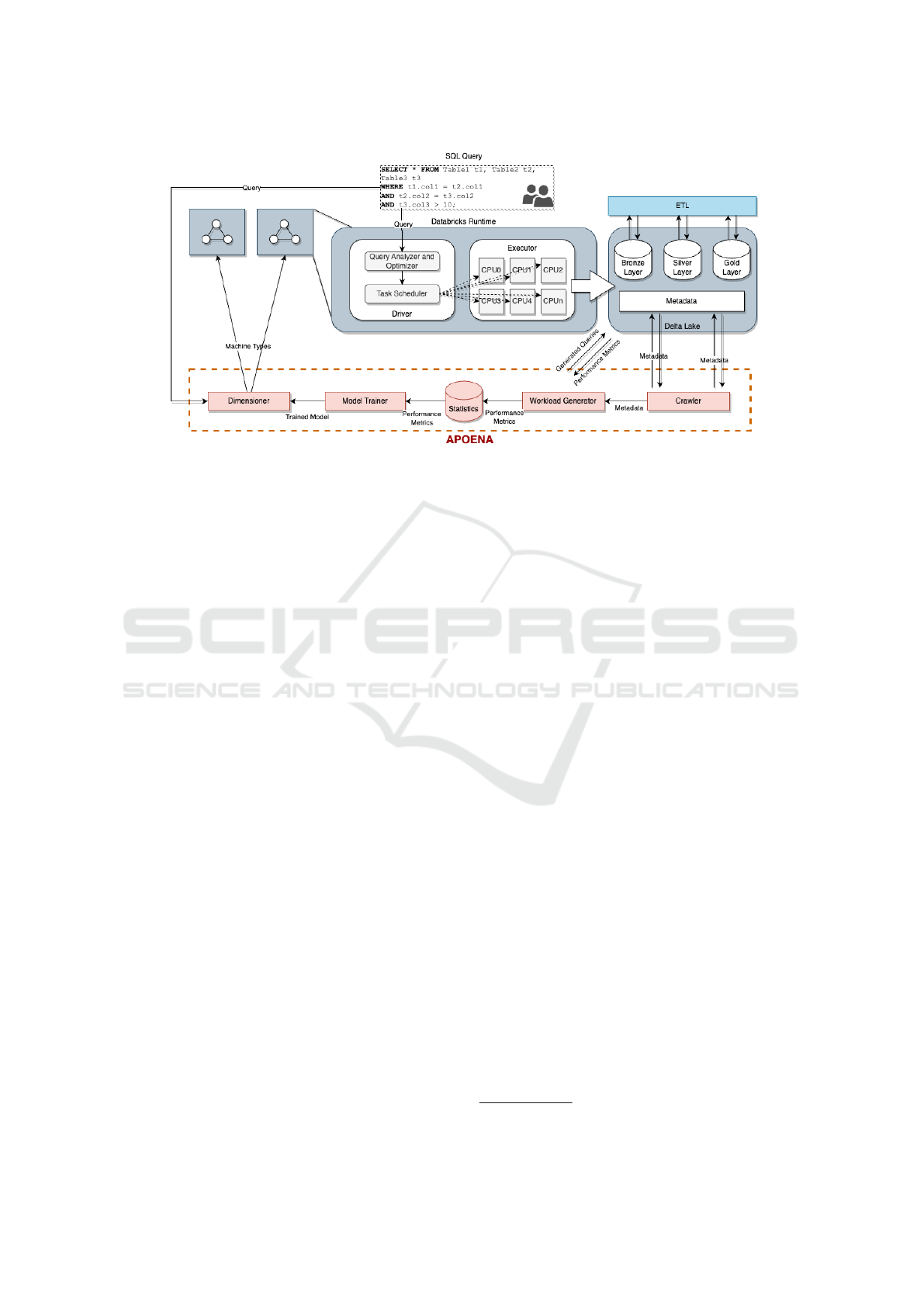
Figure 1: The Architecture of APOENA middleware. Gray components are the ones already provided by Databricks runtime

Service and Delta Lake while red components are part of APOENA.

organized into three layers: (i) Bronze Layer, (ii)

Silver Layer, and (iii) Gold Layer. The data in the

Bronze Layer does not differ signiﬁcantly from the

raw data in the Lakehouse; the distinction lies only

in the representation, wherein data from different for-

mats are loaded into a table. Data in the Silver Layer

is already transformed and cleaned. Additionally, the

data can be enriched with more useful information,

such as replacing country name abbreviations with the

full name or obtaining the complete address of a place

based on its postal code. In the Gold Layer, data is

stored in data marts for decision-making.The layer as-

sociated with each query is captured by the Crawler.

Following this, the Crawler sends the captured

metadata to the Workload Generator. This compo-

nent is employed to generate representative queries in

case the number of past executions is small (e.g., less

than 500 past executions). Since we assume that most

of the executed queries will access data stored in the

Gold Layer, we can generate multiple representative

queries to increase the number of past executions for

APOENA. In this sense, we have adapted the algorithm

for workload generation previously proposed by Or-

tiz et al. (2015), outlined in Algorithm 1. The input

consists of a database following a star or snowﬂake

schema (i.e., the database in the Gold Layer), denoted

as D = { f ∪ {dim

, dim

, ...,dim

}}, comprising one

fact table ( f ) and multiple dimension tables. It is

noteworthy that we assume the fact table has multiple

foreign keys to dimension tables. Each table t

∈ D is

composed of a set of attributes Att(t

). The algorithm

produces a set of possible queries Q to be executed

and the associated performance metrics M collected

(the generated queries may not represent a real-world

analysis to be performed by users, but it can be used

as an example for training the ML models following).

Each q

∈ Q is associated with a tuple (T

, A

, e

))

where T

is the set of tables in the FROM clause (i.e.,

the fact table and one or more dimension tables), A

is the set of projected attributes in the SELECT clause,

and e

is the selectivity factor. As previously deﬁned

by Ortiz et al. (2015), the algorithm keeps a list L with

all representative sets of tables T

. Initially, every sin-

gle table t

∈ D is inserted into L (lines 4-6), then the

algorithm generates the joins (line 8). When all rep-

resentative queries are produced, the algorithm starts

executing each q

∈ Q using different cluster conﬁgu-

rations, i.e., different types of VMs (lines 26-28).

The collected provenance data for each query exe-

cution includes: (i) query ID, (ii) number of input tu-

ples, (iii) number of output tuples, (iv) number of vC-

PUs in the worker, (v) memory (in GB) of the worker,

(vi) selectivity factor, (vii) number of workers, (viii)

number of attributes, (ix) if the query was accelerated

using Photon, (x) if the query has an inner join, (xi) if

the query has a left join, (xii) the layer (i.e., bronze,

silver, or gold), (xiii) if the query has a GROUP BY

clause, and (xiv) the execution time. Once all prove-

nance data regarding the executed queries is available,

the Model Trainer can be invoked. The Model Trainer

uses the received provenance data to train ML models

for use in the cloud dimensioning task. In its current

version, APOENA uses Linear Regression (LiR), Logis-

tic Regression (LoR), Decision Tree Classiﬁer (DTC),

and Random Forest Regression (RFR), all available in

scikit-learn

. LiR aims to ﬁt the results into a linear

https://scikit-learn.org/stable/

ICEIS 2024 - 26th International Conference on Enterprise Information Systems

292

Algorithm 1: Workload Generation.

1 Q ← {};

2 L ← {};

3 M ← {};

4 foreach t

∈ D do

5 T

← {t

};

6 L ← L ∪ T

;

7 if isFact(t

) then

8 SortDesc({dim

, ..., dim

}), 1 ≤ i ≤ k;

9 foreach j, 1 ≤ j ≤ k do

10 D

← ﬁrst j tables from D;

11 T

← T

∪ D

;

12 L ← L ∪ T

;

13 end

14 end

15 end

16 foreach T

∈ L do

17 SortDesc(Att(T

)), Att

) ≤ j ≤ Att(T

);

18 foreach k, 1 ≤ k ≤ Att(T

) do

19 A

← ﬁrst k attributes from Att(T

);

20 foreach e

∈ E

21 Q ← Q ∪ (T

, A

, e

));

22 end

23 end

24 end

25 foreach q

∈ Q do

26 foreach vm

∈ VM do

27 P

← Per f (q

, vm

);

28 M ← M ∪ P

;

29 end

30 end

equation by minimizing the sum of the squared dif-

ferences between predicted and actual values (Russell

and Norvig, 2020). Unlike LiR, LoR works with one

or more independent variables based on ﬁnding a re-

lationship between them. DTC is based on learning

the ﬁnal classiﬁcation according to its features, devel-

oping a prediction model with rules based on previ-

ous results (Russell and Norvig, 2020). Finally, RFR

comprises sample groups of decision tree classiﬁers

that estimate an average classiﬁer according to each

sample (Russell and Norvig, 2020).

Once the ML models are trained, the Dimensioner

can be invoked. The idea behind the Dimensioner

is that every time a new query is submitted, APOENA

identiﬁes the characteristics of this query and com-

bines them with all possible virtual cluster conﬁgura-

tions (i.e., the types and number of VMs). Each com-

bination of query and environment setup is then sub-

mitted to each trained ML model for inference. The

ML model responds with the expected execution time

of the query for that speciﬁc virtual cluster conﬁg-

uration. The Dimensioner then orders and presents

the top K conﬁgurations that will execute the query

faster and/or with less ﬁnancial cost, depending on the

goal deﬁned by the user. The user can then dimen-

sion the environment by choosing the most suitable

virtual cluster conﬁguration. It is worth mentioning

that APOENA does not replace any existing mechanism,

such as autoscaling. Instead, the idea is to avoid un-

necessary deployments and undeployments of VMs in

the process and to assist especially non-expert users.

4 EXPERIMENTAL EVALUATION

This section evaluates APOENA in a real production

scenario. First, we present the chosen evaluation met-

rics. Then, we discuss how the computational envi-

ronment was conﬁgured. Following that, we present

the data used in the experiments, and ﬁnally, we dis-

cuss the achieved results.

4.1 Metrics

Metrics must be employed to evaluate the perfor-

mance of trained ML models to predict the query ex-

ecution time for a speciﬁc query and virtual cluster

conﬁguration. They include True Positive (TP), True

Negative (TN), False Positive (FP) and False Nega-

tive (FN). A TP is a result in which the model cor-

rectly predicts the correct class. Similarly, a TN is a

result in which the model correctly predicts the neg-

ative class. An FP is a result in which the model in-

correctly predicts the positive class. A FN is a result

in which the model incorrectly predicts the negative

class. Based on that, we can deﬁne the Accuracy as

the number of correct predictions (TP+TN) divided

by the total of predictions (TP+TN+FP+FN). We can

also use the F1 score, which represents the harmonic

mean between precision (Precision =

T P

T P+FP

) and re-

call (Recall =

T P

T P+FN

), as deﬁned by F1 score =

2 ×

Precision×Recall

Precision+Recall

. However, the F1 score can in-

volve a micro, macro, or weighted average. Accord-

ing to Plaue, the micro average is a global metric

that considers the total of true positives, false nega-

tives, and false positives, as F1 micro =

T P

T P+

FP+FN

On the other hand, the macro average is not a global

metric. It calculates the F1 score for each class i

and determines their unweighted mean, where n is

the number of classes as deﬁned by F1 macro =

∑

i=1

F1 score

. Thus, it ignores unbalanced data. Fi-

nally, the weighted average considers unbalanced

data, calculating a F1 score for each class i separately

and its respective weight w

(Kundu, 2022), such that:

Quantity o f samples in class i

Total quantity o f samples

, thus F1 weighted =

∑

i=1

× F1 score

APOENA: Towards a Cloud Dimensioning Approach for Executing SQL-like Workloads Using Machine Learning and Provenance

293

4.2 Environment Setup

When conﬁguring the environment, the user has to

choose a plethora of parameters in Databricks plat-

form, such as the Databricks runtime version, Photon

acceleration, number of workers and VM types to be

deployed. Our experiments are based on Databricks

version 12.2 LTS (using Scala 2.12 and Spark 3.3.2).

The VM types used are a subset of the ones provided

by AWS

. We considered only the information about

the number of vCPUs, RAM (in GB) and storage size

(in GB) of each VM type. Among many options,

the chosen ones were selected based on the best cost-

beneﬁt, as presented in Table 1.

Table 1: Chosen AWS VM Types.

VM type vCPU RAM (GB) Storage (GB)

r5d.xlarge 4 32 1 x 150

r5d.2xlarge 8 64 1 x 300

i3.xlarge 32 32 1 x 950

m5d.4xlarge 64 64 2 x 300

4.3 Experiment Setup

All data used in the experiments were collected from

real-world SQL-like queries submitted to Databricks

in a large-scale company. The queries are associ-

ated with LinkedIn proﬁle data and Internal Revenue

Service data. Such data sources provide rich infor-

mation that helps data analysts determine the proﬁle

of companies and individuals based on the provided

content. The used database includes the following at-

tributes: (i) employer identiﬁcation number, (ii) share

capital, (iii) address, (iv) number of employees, (v)

business segment, (vi) revenue, (viii) email, (ix) tele-

phone number, etc. It is worth mentioning that the

used data did not have sensitive information.

A set of provenance data associated with each

query execution was collected so it is possible to

conduct the evaluations and can be divided into four

classes: (i) query structure (i.e., p-prov), (ii) con-

sumed/produced data information (i.e., r-prov), (iii)

Databricks setup and (iv) computational environment

(i.e., r-prov). Metadata regarding the query struc-

ture was collected by analyzing each query indi-

vidually to retrieve information about the usage of

speciﬁc SQL statements, such as constraints, CTE,

CASE WHEN, joins (e.g., INNER JOIN, LEFT JOIN,

and RIGHT JOIN), GROUP BY, subqueries, EXPLODE

and the selectivity factor. The latter is calculated by

determining the proportion of the ﬁltered data ana-

lyzed against the total number of tuples in the tables.

Metadata about the tables was collected, including

https://aws.amazon.com/ec2/instance-types/

the number of input rows, input and output attributes

(i.e., projection). Concerning the computational en-

vironment and the number of vCPUs information in

each VM, the RAM amount (in GBs) in each VM and

the storage capacity (in GBs) in each VM were gath-

ered. Finally, concerning the Databricks setup, infor-

mation on the number of workers, the type of each

worker and whether the query used Photon for accel-

eration was collected.

We also specify the ML algorithms that will be

employed to train the ML models by APOENA. Since

we are using scikit-learn as the ML framework, we

have chosen the following algorithms: LiR, LoR,

DTC and RFR. Each trained ML model is submitted

to the 10-fold Cross-Validation method for evaluation

of the F1 weighted metric.

4.4 Results

Since in APOENA, we aim to predict the execution time

of a SQL-like query based on characteristics of the

query and the computational environment used, the

query execution time is our target class. As the execu-

tion time of queries is rarely the same, it is preferable

to discretize this class into a series of execution time

intervals. Our ﬁrst task is to choose a suitable number

of intervals for query execution time. Table 2 presents

eight possible discretizations of the query execution

time that can be used by APOENA.

The dataset, containing query provenance and

Databricks environment features, becomes unbal-

anced depending on chosen execution time intervals.

Real-world data from a production system shows

the majority of queries execute in under 600 sec-

onds. Thus, fewer intervals lead to a more unbalanced

dataset, with most queries falling into the ﬁrst inter-

val. Hence, we evaluate scenarios with six, seven, and

eight execution time intervals. Figure 2(a) shows the

percentage of examples per time interval for a sce-

nario with eight intervals.

After deﬁning the number of execution time inter-

vals, we evaluated the importance of features in the

dataset. Selecting the most relevant features based

on their impact on the predicted result is essential for

APOENA. Measures based on the impurity reduction of

splits in DTC are common since they are simple and

fast to compute. Thus, we have chosen to use Gini im-

portance (Nembrini et al., 2018). Figure 2(b) presents

the importance of each feature.

Differently from what we expected, some features

presented low importance in the dataset, such as the

use of LEFT JOIN and INNER JOIN clauses in the

queries. This could be due to the fact that only one

query includes a LEFT JOIN, which reduces its global

ICEIS 2024 - 26th International Conference on Enterprise Information Systems

294

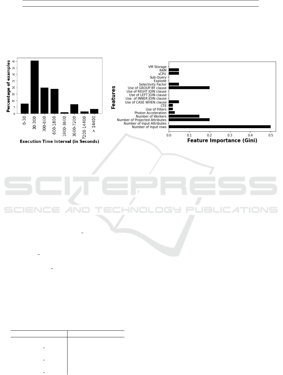
Table 2: Intervals for Query Execution Time (in seconds).

Number of Intervals Intervals (in seconds)

2 0-1800; > 1800

3 0-300; 300-3600; > 3600

4 0-300; 300-1800; 1800-7200; > 7200

5 0-300; 300-1800; 1800-7200; 7200-14400; > 14400

6 0-300; 300-1800; 1800-3600; 3600-7200; 7200-14400; > 14400

7 0-300; 300-600; 600-1800; 1800-3600, 3600-7200; 7200-14400; > 14400

8 0-30; 30-300; 300-600; 600-1800; 1800-3600; 3600-7200; 7200-14400; > 14400

Figure 2: (a) Percentage of examples per execution time interval (8 intervals). (b) Feature Importance.

importance despite adding to the complexity of that

query. However, as expected, the number of tuples

processed by the query and characteristics of the envi-

ronment, e.g., the number of vCPUs, and the number

of workers have an impact on the result. All features

with importance greater than zero were considered in

the following analyses.

We have executed each ML algorithm to train the

models for 6, 7, and 8 execution time intervals, eval-

uating the accuracy and the F1 weighted metrics of

each one. By analyzing Table 3, one can observe that

the DTC is the classiﬁer that showed the highest ac-

curacy and F1 weighted for all three execution time

intervals. We have set the minimum accepted values

for accuracy and F1 weighted at 0.9 for both metrics.

Therefore, the DTC was the chosen ML model for use

in this dataset by APOENA. It is worth noting that a dif-

ferent classiﬁer may be chosen if the query patterns

change drastically over time. Thus, the ML models

have to be retrained periodically in APOENA. The au-

tomatic retraining feature is still under development.

Table 3: Performance metrics according to time intervals.

Intervals Metric LiR LoR RFR DTC

Accuracy 0.70 0.36 0.88 0.94

F1 weighted 0.77 0.19 0.91 0.94

Accuracy 0.46 0.22 0.80 0.84

F1 weighted 0.57 0.08 0.81 0.84

Accuracy 0.42 0.22 0.64 0.76

F1 weighted 0.48 0.08 0.67 0.76

We also assessed the impact of correct and incor-

rect recommendations made by APOENA for two rep-

resentative queries (transformations from bronze to

the silver layer). The ﬁrst one accessed 332,263,103

tuples, producing 41,041,580 tuples as output. This

query is executed in a virtual cluster composed of

two VMs r5d.2xlarge for 1,219 seconds. APOENA cor-

rectly classiﬁed it into the 300-1800 execution time

interval and the query was executed within the pre-

dicted time, costing US$ 4.87. On the contrary, the

second one accessed 1,327,822,307 tuples, producing

415,478,474.00 tuples as output. The optimal con-

ﬁguration for a balance of performance and cost was

a virtual cluster composed of 10 VMs m5d.4xlarge,

running for 1,776.00 seconds and costing approxi-

mately US$ 35.52. However, APOENA classiﬁed the

execution time interval for this query as 14,400 sec-

onds, which may make the user choose a different

virtual cluster conﬁguration. We only considered the

VM types presented in Table 1. If more powerful

VMs are available for APOENA, the user might choose

an over-dimensioned conﬁguration incurring higher

ﬁnancial costs. Finally, we evaluated the overhead

imposed by APOENA to dimension the virtual cluster.

On average, APOENA needed 100 seconds to train ML

models and less than a second for inference, which

can be considered an acceptable overhead.

APOENA: Towards a Cloud Dimensioning Approach for Executing SQL-like Workloads Using Machine Learning and Provenance

295

5 CONCLUSIONS

Several big data processing platforms have emerged,

with Databricks standing out as one of the most

prominent options. It offers a range of cloud-based

services for executing complex queries and transac-

tional workloads. However, it requires the dimen-

sioning of the cloud environment, demanding users to

specify the types and number of VMs for deployment,

a task that can be far from trivial. Identifying the

characteristics of a SQL-like workload and estimat-

ing the appropriate VM type from a selection of more

than 100 options poses a complex challenge. While

mechanisms like autoscaling exist in Databricks, they

are costly and may not be straightforward to con-

ﬁgure for non-expert users. Improperly dimension-

ing the cloud environment, either through over or

under-dimensioning, can impact both workload per-

formance and ﬁnancial costs.

This paper proposes a middleware named APOENA,

designed to dimension the cloud environment for spe-

ciﬁc workloads, i.e., SQL-like queries. APOENA col-

lects provenance data and employs this historical data

to train ML models capable of predicting query per-

formance for a particular combination of a query and

virtual cluster conﬁguration. This conﬁguration in-

cludes the type and number of VMs involved in the

execution. Although APOENA focused on Databricks

in this paper, it could be extended to work with other

big data frameworks such as Apache Spark.

Experiments with real-world workloads demon-

strated that APOENA classiﬁed query execution times

with over 90% accuracy and F1 weighted met-

rics. Future work involves implementing a retraining

mechanism for APOENA, as the current version does

not perform retraining automatically. Additionally,

we plan to evaluate APOENA using a broader range of

real-world workloads.

ACKNOWLEDGMENTS

This study was ﬁnanced in part by the Coordenac¸

de Aperfeic¸oamento de Pessoal de N

ıvel Superior

- Brasil (CAPES) - Finance Code 001. This pa-

per was also partially ﬁnanced by CNPq (grant

311898/2021-1) and FAPERJ (grant n

E-

26/202.806/2019).

REFERENCES

Ahmed, N. et al. (2022). Runtime prediction of big data

jobs: performance comparison of machine learning al-

gorithms and analytical models. J. Big Data, 9(1):67.

Armbrust, M. et al. (2020). Delta lake: High-performance

ACID table storage over cloud object stores. Proc.

VLDB Endow., 13(12):3411–3424.

Behm, A. et al. (2022). Photon: A fast query engine for

lakehouse systems. In SIGMOD’22, pages 2326–

2339. ACM.

Burdakov, A. et al. (2020). Predicting sql query execu-

tion time with a cost model for spark platform. In

IoTBDS’20, pages 279–287. INSTICC, SciTePress.

de Oliveira, D. E. M. et al. (2021). Towards optimizing the

execution of spark scientiﬁc workﬂows using machine

learning-based parameter tuning. Concurr. Comput.

Pract. Exp., 33(5).

Filho, E. R. L., de Almeida, E. C., Scherzinger, S., and

Herodotou, H. (2021). Investigating automatic param-

eter tuning for sql-on-hadoop systems. Big Data Res.,

25:100204.

Groth, P. and Moreau, L. (2013). W3C PROV - An

Overview of the PROV Family of Documents. Avail-

able at https://www.w3.org/TR/prov-overview/.

Herschel1, M., Diestelk

amper1, R., and Lahmar, H. B.

(2017). A survey on provenance: What for? what

form? what from? The VLDB Journal.

Kundu, R. (2022). F1 score in machine learning: Intro &

calculation.

Meredino, A. et al. (2018). Big data, big decisions: The im-

pact of big data on board level decision-making. Jour-

nal of Business Research.

Mustafa, S., Elghandour, I., and Ismail, M. A. (2018). A

machine learning approach for predicting execution

time of spark jobs. Alexandria Engineering Journal,

57(4):3767–3778.

Nargesian, F., Pu, K. Q., Bashardoost, B. G., Zhu, E., and

Miller, R. J. (2023). Data lake organization. IEEE

Trans. Knowl. Data Eng., 35(1):237–250.

Nembrini, S., K

onig, I. R., and Wright, M. N. (2018).

The revival of the gini importance? Bioinform.,

34(21):3711–3718.

Ortiz, J., de Almeida, V. T., and Balazinska, M. (2015).

Changing the face of database cloud services with per-

sonalized service level agreements. In CIDR’15.

Ozt

urk, M. M. (2023). Tuning parameters of apache

spark with gauss–pareto-based multi-objective opti-

mization. Knowledge and Information Systems.

Plaue, M. (2020). Data Science - An Introduction to Statis-

tics and Machine Learning. Springer.

Russell, S. J. and Norvig, P. (2020). Artiﬁcial Intelligence:

A Modern Approach (4th Edition). Pearson.

Singhal, R. and Nambiar, M. (2016). Predicting sql query

execution time for large data volume. In IDEAD’16,

page 378–385, New York, NY, USA. Association for

Computing Machinery.

Zaharia, M. (2019). Lessons from large-scale software as a

service at databricks. In SoCC’19, page 101.

Zaharia, M. et al. (2021). Lakehouse: A new generation

of open platforms that unify data warehousing and ad-

vanced analytics. In CIDR’21. www.cidrdb.org.

ICEIS 2024 - 26th International Conference on Enterprise Information Systems

296