Optimal Velocity Model Based CACC Controller for Urban Scenarios
Anas Abulehia, Reza Dariani
a
and Julian Schindler
b
Institute of Transportation Systems, German Aerospace Center (DLR), Braunschweig, Germany
Keywords:
CCAC, Optimal Velocity Model, Linear Quadratic Controller.
Abstract:
To address the current high level of congestion, a connected vehicle system in the form of a platoon or Co-
operative Adaptive Cruise Control (CACC) presents a promising solution. This system significantly reduces
stop-and-go traffic, as well as fuel consumption. A Cooperative Adaptive Cruise Control (CACC) system com-
prises two or more closely-following vehicles traveling at a desired cruising velocity and distance headway.
Compared with human drivers, such a system has the advantage of reducing inter-vehicle distance, making it a
promising solution for mitigating traffic congestion as well as reducing aerodynamic drag, and fuel consump-
tion. This work aims to introduce a new Cooperative Adaptive Cruise Control (CACC) based on the optimal
velocity model in traffic dynamics. Several controllers for the introduced CACC system will be presented,
particularly various versions of the linear quadratic controller. Simulation scenarios for these controllers will
also be discussed.
1 INTRODUCTION
Mobility is indispensable in human life, impacting
various aspects from daily commutes to exploring
distant tourist destinations. It is an integral part of
our existence. Globally, in 2012, the average dis-
tance traveled per person was 7,000 miles annually.
Over 80% of this travel occurred in vehicles, includ-
ing cars, taxis, buses, and similar modes of transporta-
tion (Brand et al., 2019).
Tackling traffic jams is challenging because, in
many cases, no clear reason for the emergence of new
congestion is found. A false braking incident some-
where could be propagated and transformed into a
traffic jam. A driving assistance system like Coop-
erative Adaptive Cruise Control (CACC) offers a so-
lution to the traffic problem. The main advantage of
CACC is improving traffic flow and reducing traffic
congestion. Other benefits include enhanced safety
and comfort when compared with other vehicular sys-
tems. According to (Shladover et al., 2015), the time
gap can be reduced from about 1.4 to 0.6 seconds
when using CACC.
The CACC concept is the combination of auto-
mated speed control with a cooperative element, such
as Vehicle-to-Vehicle (V2V) and/or Infrastructure-
to-Vehicle (I2V) communication (Shladover et al.,
a
https://orcid.org/0000-0002-1091-8793
b
https://orcid.org/0000-0001-5398-8217
2015). The literature of CACC system is well estab-
lished in the scientific community. In (Wang et al., ) a
review on CACC system was presented. Framing our
work within it , the flow of information is considered a
vehicle parameter, allowing for various possible infor-
mation flow topologies. Although the simulation sec-
tion focuses on three specific topologies, it’s impor-
tant to note that bidirectional information flow is not
defined; the system permits information to go down-
stream only. The control problem has been addressed
individually for each vehicle without employing any
centralization concept.
In addressing challenges, recent works such as
those (Hsueh et al., 2022), (Bekiaris-Liberis, 2023),
(Xing et al., 2022), (Fu et al., 2023) have been ded-
icated to mitigating the impact of time delay, which
can adversely affect the performance of any baseline
CACC. Furthermore, there is a growing emphasis on
enhancing the robustness and security of the system
against communication degradations or attacks. (Liu
et al., 2023), (Yang et al., 2023), and (Zhongwei et al.,
) have contributed significantly to this area, reflecting
the maturation of CACC technology.
This paper focuses on the V2V CACC system.
The first section of this paper discusses the CACC
system using the Optimal Velocity Model, and the
MOTIF concept is introduced. Central Optimal Con-
trol has been addressed by (Ge and Orosz, 2016). The
second section deals with the control problem at the
Abulehia, A., Dariani, R. and Schindler, J.
Optimal Velocity Model Based CACC Controller for Urban Scenar ios.
DOI: 10.5220/0012650200003702
Paper published under CC license (CC BY-NC-ND 4.0)
In Proceedings of the 10th International Conference on Vehicle Technology and Intelligent Transport Systems (VEHITS 2024), pages 327-335
ISBN: 978-989-758-703-0; ISSN: 2184-495X
Proceedings Copyright © 2024 by SCITEPRESS – Science and Technology Publications, Lda.
327

vehicle level (decentralized). The Linear Quadratic
Regulator was utilized with different variations. The
third section shows closed-loop simulations of differ-
ent scenarios.
2 OPTIMAL VELOCITY MODEL
The Optimal Velocity model (Bando et al., 1994),
(Bando et al., 1995), is a single-lane mathematical
traffic model. It models traffic using physically mean-
ingful parameters. The model describes traffic con-
gestion by analyzing the behavior of each individual
vehicle, utilizing the headway between preceding and
following vehicles to compute the following vehicle’s
velocity. The model has garnered significant scien-
tific attention due to its stability in both analytical
and numerical analyses. The Optimal Velocity Model
surpasses other models in terms of its simplicity and
meaningful parameters, which have a physical basis,
unlike other models with non-physical parameters.
Figure 1: car following notation, image source(Reimann,
2008).
Figure 1 shows two successive vehicles on a road,
where s,v,L denote distance progress, velocity, and
bumper-to-bumper length of vehicles i and i − 1.
∆s
i
(t) = s
i−1
(t) − s
i
(t) − L
i−1
(1)
The distance between two vehicles on the road is de-
fined by equation 1. ∆s
i
(t) is also defined as the head-
way distance h
i
(t).
The state variables of the Optimal Velocity Model
are headway distance h
i
(t) and velocity v
i
(t). The Op-
timal Velocity Model of a vehicle i can be expressed
in the form of the following nonlinear equations.
˙
h
i
(t) = v
i−1
(t) − v
i
(t)
˙v
i
(t) = F

h
i
(t − τ),
˙
h
i
(t − τ), v
i
(t − τ)

(2)
Equation 2 indicates that the change in headway of
a vehicle is influenced by its velocity and the veloc-
ity of the preceding vehicle. It models the accelera-
tion of the vehicle i as a nonlinear function F of the
time-shifted headway, the time derivative of the head-
ing, and the vehicle’s velocity. The introduced time
shift τ is meant to compensate for all incurred delays,
with the most significant being the driver’s reaction
time. In this work, it is neglected as the system is
automated. The nonlinear function F describes the
vehicle’s velocity state evolution. The definition of F
is given in Equation 3.
F(h
i
,
˙
h
i
,v
i
) = α(V (h
i
) − v
i
) + β
˙
h
i
(3)
The variables α and β are control gains corre-
sponding to the link between vehicle i and i − 1.The
selection of these parameters is very important and
should be carefully studied, taking into consideration
the vehicle capabilities. The function V defines the
continuous range policy that commands the vehicle
velocity and is known as the range policy, defined
based on two boundary variables h
st
the stop headway
and h
go
the free speed headway. They represent the
minimum headway distance the vehicle should main-
tain and the maximum headway distance at which the
velocity of the vehicle is v
max
.
V (h) =



0 if h
i
≤ h
st
f
v
(h
i
) if h
st
< h
i
< h
go
v
max
if h
i
≥ h
go
(4)
Indeed, many possible functions can be intro-
duced to achieve an increasing piecewise function; in
(Zhang and Orosz, 2013), three candidates of f
v
(h
i
)
were presented.
f
v1
(h
i
) = v
max
h
i
− h
st
h
go
− h
st
,
f
v2
(h
i
) =
v
max
2

1 − cos

π
h
i
− h
st
h
go
− h
st

,
f
v3
(h
i
) =
v
max
2

1 + tanh

tan

π
2
2h
i
− h
go
− h
st
h
go
− h
st

,
(5)
Among these, f
v1
is not a suitable option since it
does not yield a continuous derivative function. Non-
smooth transitions occur at h
st
and h
go
, leading to dis-
continuities in the jerk and discomfort for the driver.
Therefore, f
v1
is ruled out. Both f
v2
and f
v3
exhibit
very similar behaviors. Up to this point, the intro-
duced model incorporates only two vehicles. An en-
hancement to the model is proposed in (Zhang and
Orosz, 2015). They introduce the MOTIF biologi-
cal concept with some modifications. The concept,
used as a vehicle MOTIFm, observes the states of the
immediate vehicle ahead, as well as the m-th vehi-
cle ahead. This requires velocity value of the vehicle
i, preceding vehicle i − 1 and the m-th vehicle ahead
i − m.
It also requires headway value of vehicle’s head-
way h
i
, and all headway values of the vehicles from
i − m + 1 to i.
VEHITS 2024 - 10th International Conference on Vehicle Technology and Intelligent Transport Systems
328

˙
h
i
(t) =v
i−1
(t) − v
i
(t),
˙v
i
(t) =α
1
(V (h
i
(t)) − v
i
(t)) + β
1
(v
i−1
(t) − v
i
(t))+
α
m
V
1
m
i
∑
k=i−m+1
h
k
(t)
!
− v
i
(t)
!
+
β
m
(v
i−m
(t) − v
i
(t))
(6)
As observed in (6), the velocity of vehicle i relies on
the variables v
i
, v
i−1
, v
i−m
, h
i
, and the average of h
from the vehicle i to vehicle i − m +1. Equation (6) is
designateed as the optimal velocity model. As previ-
ously mentioned, given the non-linear function V de-
fined in (4), the model linearization around a chosen
equilibrium point is proceeded.
2.1 Linearization of the Optimal
Velocity Model
This section outlines the linearization process of (6).
The linearization is performed around a specific point
known as an equilibrium point, which characterizes
the system dynamics within the vicinity of an oper-
ational boundary. This step is imperative for linear
control approaches in system analysis and control.
The equilibrium point is represented by h
∗
i
and v
∗
i
.
The system states h
i
,v
i
are expressed in relation to
the equilibrium point, with the headway defined as
h
i
= h
∗
i
+
˜
h
i
and the velocity as v
i
= v
∗
i
+ ˜v
i
. The
tilde symbol signifies the deviation of the vehicle state
from the equilibrium point. The first two terms of the
Taylor’s approximation are considered.
Let’s take the first equation from (6) and substitute
all variables relative to the operating point.
According to Taylor expansion, any function can
be approximated
f (x) = f (x
∗
) +
f
′
(x
∗
)
1!
(x − x
∗
)+
f
′′
(x
∗
)
2!
(x − x
∗
)
2
+
f
′′′
(x
∗
)
3!
(x − x
∗
)
3
+ · · · ,
(7)
In order to linearize the system only the first two
terms of the equation should be considered. Taking
the first state equation from (6), it is rewritten relative
to the operating point, resulting in
˙
h
i
= v
i−1
− v
i
d(h
∗
+
˜
h
i
)
dt
= v
∗
i−1
+ ˜v
i−1
− v
∗
i
+ ˜v
i
(8)
Since h
∗
and v
∗
are constant, the equation becomes
˙
˜
h
i
= ˜v
i−1
− ˜v
i
(9)
Similarly, the second state v
i
is linearized.
˙v
i
= f

v
∗
i−1
,v
∗
i
,h
∗
i
,v
∗
i−m
,h
∗
i−m+1
,h
∗
i−m+2
,...,h
∗
i−1

+
∂ f (v
∗
i−1
)
∂v
i−1
( ˜v
i
) +
∂ f (v
∗
i−m
)
∂v
i
( ˜v
i
) +
∂ f (h
∗
i
)
∂h
i
(
˜
h
i
)
+
∂ f (h
∗
i−m
)
∂v
i−m
( ˜v
i−m
) +
∂ f (h
∗
i−m+1
)
∂h
i−m+1
(
˜
h
i−m+1
)
+
∂ f (h
∗
i−m+2
)
∂h
i−m+2
(
˜
h
i−m+2
) + · · · +
∂ f (h
∗
i
)
∂h
i
(
˜
h
i
)
(10)
The partial derivatives are given in equation 11.
∂ f
∂v
i−1
= β
1
,
∂ f
∂v
i
= −β
m
− β
1
− α
1
− α
m
∂ f
∂h
i
= α
1
V
′
(h
∗
i
),
∂ f
∂v
i−m
= β
m
∂ f
∂h
i−m+1
=
α
m
m
V
′

h
∗
i−m+1

,
∂ f
∂h
i−m+2
=
α
m
m
V
′

h
∗
i−m+2

,· · · ,
∂ f
∂h
i
=
α
m
m
V
′
(h
∗
i
)
(11)
The below equation 12 describes the linearized sys-
tem.
˙
˜
h
i
= ˜v
i−1
− ˜v
i
˙
˜v
i
=β
1
˜v
i−1
− (α
1
+ β
1
+ α
m
+ β
m
) ˜v
i
+ α
1
V
′
˜
h
i
+ β
1
˜v
i−m
+
α
m
V
′
˜
h
i
m
+
α
m
V
′
m

˜
h
i−1
+
˜
h
i−2
+ ... +
˜
h
i−m+1

(12)
The system of linear equations in equation 13
describes the dynamics of the enhanced CACC of
MOTIFm when m > 1. In the case of m = 1, all pa-
rameters with m subscript are set to zero. Table 1 lists
all numerical values of the OVM parameters used for
analytical analysis and numerical simulation.

˙
˜
h
i
˙
˜v
i

=

0 −1
α
1
V
′
+
α
m
V
′
m
− (α
1
+ α
m
+ β
1
+ β
m
)

˜
h
i
˜v
i

+

1
β
1

˜v
i−1
+

0
β
m

˜v
i−m
+

0
α
m
V
′
m

i−1
∑
k=i−m+1

˜
h
k

+

0
1

˜u
˜y =

1 0


˜
h
i
˜v
i

(13)
Optimal Velocity Model Based CACC Controller for Urban Scenarios
329

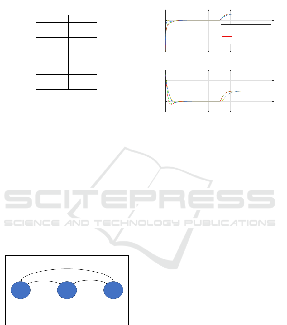
Table 1: Optimal Velocity Model Parameters.
Parameter Value
α
1
2
α
m
2
β
1
2
β
m
2
V
′
π
2
h
∗
i
20 [m]
v
∗
i
15 [m/s]
h
st
5 [m]
h
go
35[m]
2.2 Linearized Model Validity
In this section the accuracy of the linearized model is
investigated.
To this end, a simple Cooperative Adaptive Cruise
Control (CACC) system consisting of three vehicles
is defined. The leading vehicle denoted as i = 0, will
not be investigated as it is not an Optimal Velocity
Model (OVM) vehicle and is modeled as a linear first-
order system. The middle vehicle denoted as i = 1, is
considering only one vehicle ahead i.e it has MOTIF1,
and the last vehicle, denoted as i = 2, is considering
two vehicles ahead i.e it has MOTIF2, as depicted in
the figure 2.
A scenario with states far from the linearization
point, i.e., h
∗
and v
∗
, is defined where the initial states
are h
1
,h
2
equal to 25[m] and v
1
,v
2
equal to 0. The
leading vehicle starts moving, and states are com-
pared between both the nonlinear OVM equation (8)
and the linearized OVM (12). As shown in the figure
3.
Vehicle 0Vehicle 1Vehicle 2
Figure 2: Linearized Model Fidelity Vehicles’ Diagram.
To quantify the model validity, the mean squared
error is computed. As shown in Figure 3 and Ta-
ble 2, there is only a minimal deviation between the
linearized and non-linear OVM models despite the
simulation scenario starting far from the linearization
point. This observation suggests that the model is
highly faithful.
0 10 20 30 40 50
Time [s]
0
5
10
15
20
Velocity [m/s]
Vehicle 1 (linear)
Vehicle 2 (linear)
Vehicle 1(nonlinear)
Vehicle 2 (nonlinear)
0 10 20 30 40 50
Time [s]
18
20
22
24
26
Headway [m]
Figure 3: The System States of the Linearized and Nonlin-
ear Model.
Table 2: Mean Squared Error Of The Fidelity Scenario.
State MSE
v
1
0.0052 [m
2
/s
2
]
v
2
0.0061 [m
2
/s
2
]
h
1
0.0124[m
2
]
h
2
0.0041[m
2
]
3 CONTROLLER DESIGN
The Linear-Quadratic Regulator (LQR) problem is a
control problem in which an optimal control law is
sought for a linear time-invariant system subject to
quadratic cost criteria. The objective is to minimize
a quadratic cost function that includes the system’s
states and control inputs. There are two methods
for finding the solution to the linear quadratic regula-
tor problem: Dynamic Programming (Bellman, 1966)
and the Pontryagin method (Pontryagin, 1987).
In his dissertation (Nguyen and Bestle, 2007),
Nguyen presented a well-documented and complete
solution to the linear quadratic regulator problem with
disturbances by applying the Pontryagin principle.
3.1 Linear Quadratic Regulator
Here, the problem of the linear quadratic regulator
with disturbances is defined and found its solution.
Considering a linear time-invariant system with af-
fecting disturbances on the states and measurement
model.
˙x = Ax + Bu + B
w
w, x(0) = x
0
y = Cx + Du + D
w
w
(14)
VEHITS 2024 - 10th International Conference on Vehicle Technology and Intelligent Transport Systems
330

where the vectors x ∈ R
n
,y ∈ R
m
,u ∈ R
p
,w ∈ R
q
represent the states, the measured outputs, the con-
trol inputs and the disturbance input respectively.
The matrices A ∈ R
n×n
,B ∈ R
n×p
,C ∈ R
m×n
,D ∈
R
n×q
,B
w
∈ R
n×w
,D
w
∈ R
m×w
represent the state , in-
put, output, feed-through, input disturbance, and out-
put disturbance respectively. The objective function
defines the importance of each state of our system and
the energy used, and the cost is a quadratic function
of states x and inputs u.
J =
Z
∞
0

y
T
Q
y
y + u
T
R
u
u

dt (15)
where Q
y
≻ 0, R
u
≻ 0 are positive definite matrices
the weighting matrices of outputs and inputs, respec-
tively. The linear quadratic regulator aims to find the
input value that minimizes the objective function as in
equation 16.
min
R
∞
0

y
T
Q
y
y + u
T
R
u
u

dt
s.t. ˙x = Ax + Bu + B
w
w
(16)
J =
Z
∞
0
"
(Cx + Du + D
w
w)
T
Q
y
(Cx + Du + D
w
w) + u
T
R
u
u
#
dt
=
Z
∞
0
"
(Cx + Du)
T
Q
y
(Cx + Du)+ 2(Cx +Du)
T
Q
y
D
w
w
+ w
T
D
T
w
Q
y
D
w
w + u
T
R
u
u
#
dt
=
Z
∞
0
"
x
T

C
T
Q
y
C

| {z }
:=Q
x + 2x
T

C
T
Q
y
D

| {z }
:=N
u + u
T

D
T
Q
y
D + R
u

| {z }
:=R
u
#
dt
+
Z
∞
0
"
2x
T
C
T
Q
y
D
w
| {z }
:=N
xw
w + 2w
T
D
T
w
Q
y
D
| {z }
:=N
uw
u + w
T
D
T
w
Q
y
D
w
w
| {z }
:=R
w
#
dt
=
Z
∞
0
"
x
T
Qx + 2x
T
Nu + u
T
Ru
#
dt +
Z
∞
0
"
2x
T
N
xw
w + 2w
T
N
uw
u + w
T
R
w
w
#
dt
=:
Z
∞
0
F (u,x,w,t)dt
(17)
The equation (16) shows the complete definition
of LQR problem as an optimization problem. The so-
lution to this problem is mathematically not straight
forward, as stated before. The solution is shown. Sub-
stituting the y in the equation (16)
The control law is composed of two parts: the
state feedback term, which relates the input to the
state vector x, and the disturbance feed-forward term,
which relates the input to the disturbance vector w:
u = u
x
+ u
w
= K
x
x + K
w
w (18)
The equation (19) represents the formula for the state
feedback gain K
x
, while the disturbance feed-forward
gain K
w
is shown in (20).
K
x
= −R
−1

N
T
+ B
T
P

(19)
K
w
= −R
−1
N
uw
T
+ B
T
h
A
T
+ (K
x
)
T
B
T
i
−1
h
(K
x
)
T
N
uw
T
− (N
xw
+ PB
w
)
i
!
(20)
The matrix P, which appears in both formulas for
K
x
and K
w
, is known as the Riccati matrix. The value
of P satisfies the equality 21. Further details can be
found in (Naidu, 2002), page 129.
PA + A
T
P − (PB + N)R
−1

N
T
+ B
T
P

+ Q = 0
(21)
Upon revisiting the state space model in the equation
(13), where D and D
w
are zero, all non-(
˜
h
i
, ˜v
i
, ˜u) can
be lumped into the disturbance matrix B
w
. Conse-
quently, the control gains K
x
and K
w
take the form:
K
x
= −R
−1

B
T
P

(22)
K
w
= −R
−1
B
T
h
A
T
+ (K
x
)
T
B
T
i
−1
(PB
w
)
!
(23)
Several key points regarding the obtained control
formula are discussed in this section.
• The optimal feed-forward disturbance gain K
w
, as
shown in formula 23, depends not only on the sys-
tem definition and the assigned input cost matrix
but also on the optimal state feedback gain K
x
.
• By setting K
w
to zero, the result of an LQR is ob-
tained. In this case, the control formula does not
compensate for the measured disturbances w, but
the control is still able to keep the states still, al-
beit more slowly than when K
w
is incorporated.
• LQR does not consider the physical limits of the
system, such as saturation, making the selection
of the weighting matrices R and Q challenging.
Extensive simulations are necessary to ensure that
the controller does not push the system to its ac-
tuation limits. Other controllers, such as MPC
and the constrained LQR (Scokaert and Rawlings,
1998), perform better in this aspect.
• LQR maintains the system at a specific state when
the reference signal is 0. If the reference signal
changes or disturbances occur, a steady-state error
appears. To make the system follow the reference
input, either adding a state to the system to rep-
resent the error between the reference signal and
the output, known as state augmentation (
˚
Astr
¨
om
and Murray, 2021), or incorporating the system’s
disturbances, known as optimal disturbance feed-
forward with the gain matrix K
w
.
• The state augmentation process makes the selec-
tion of R and Q even more difficult because the
additional system state has a linear relationship
with the other states.
• Alternatively, the LQR can be used to solve the
regulating problem, whereas a manually tuned
Optimal Velocity Model Based CACC Controller for Urban Scenarios
331

gain is used to eradicate the steady-state error.
However, this means the controller is optimal in
regulating the states but not necessarily in track-
ing the input reference.
All controllers have been designed with the sys-
tem values as per table 1 for MOTIF1. For other MO-
TIF configurations, the values are α
1
= 1.5, α
m
= 1,
β
1
= 0.6, and β
m
= 0.9. This modification makes the
system matrix A for all MOTIF configurations identi-
cal. This makes one controller universal for any MO-
TIF and allows us to inspect the impact of the MOTIF
configuration on the whole system as well as the con-
troller performance.
Before finding the control gains of the state-space
model in (13), the controllability needs to be checked.
The controllability matrix C = [B, AB] should be a
full-rank matrix.

0 −1
1 −α
1
− α
m
− β
1
− β
m

(24)
The system in (13) has a full-rank controllability ma-
trix (24). Designing an LQR controller for the sys-
tem described in (13) does not yield zero steady-
state error. The controller maintains the system at a
specific state when the system is at its linearization
point. However, when the leading or preceding vehi-
cle changes its velocity, the following vehicle deviates
from the linearization point, and a steady-state error
appears. This happens because the controller does not
account for the other signals, i.e., ˜v
i−1
, ˜v
i−m
,... The
selection of the weighting matrices is an iterative pro-
cess where satisfactory system response is obtained.
The control gains can be found using MATLAB™’s
lqr function with the weighting matrices Q and R.
The control gain matrix K
x
.
K
x
= −

−16.7064 3.0365

(25)
The Riccati matrix P.
P =

123.5829 −16.7064
−16.7064 3.0365

(26)
3.2 Linear Quadratic Regulator with
Disturbance Feed-Forward
Simulations show that the Linear Quadratic Regulator
does not yield zero steady-state error. In this section,
the LQR with a disturbance feed-forward term is com-
bined. By substituting the K
x
equation (25) and the P
equation (23) in equation (23), the gain K
w
= 6.64
which is valid only for MOTIF1.
Simulation of this controller shows that it was able
to reach a zero steady-state error. Tuning of the dis-
turbance gain K
w
is not possible because it depends
on K
x
. A small change in K
w
makes the controller
not valid in that particular case, and steady-state error
appears. One last caveat is that this controller allows
the disturbance signals to propagate and be amplified
through the following vehicles even with a low K
w
value.
3.3 Linear Quadratic Regulator with
Integral Action
To ensure that the controller precisely follows the ref-
erence input, the second approach is to incorporate in-
tegral action. This involves introducing an additional
state to represent the error between the reference sig-
nal and the output a process known as Integral action
(Malkapure and Chidambaram, 2014). The new state
is defined as
˙
˜e
i
= ˜r
i
−
˜
h
i
, where ˜r
i
is the desired head-
way reference. This new state equation is added to the
state space equation (13).


˙
˜
h
i
˙
˜v
i
˙
˜e
i


=


0 −1 0
α
1
V
′
+
α
m
V
′
m
− (α
1
+ α
m
+ β
1
+ β
m
) 0
−1 0 0




˜
h
i
˜v
i
˜e
i


+


0
1
0


˜u
i
+


1
β
1
0


˜v
i−1
+


0
β
m
0


˜v
i−m
+


0
α
m
V
′
m
0


i−1
∑
k=i−m+1

˜
h
k

+


0
0
1


˜r
i
˜y =

1 0 0



˜
h
i
˜v
i
˜e
i


(27)
The controllability matrix C = [B,AB,A
2
B] in (28)
is a full rank matrix.



0 −1 α
1
+ α
m
+ β
1
+ β
m
1 −α
1
− α
m
− β
1
− β
m
(α
1
+ α
m
+ β
1
+ β
m
)
2
−V
′
α
1
−
V
′
α
m
m
0 0 1



(28)
Using the same weighting matrices as per subsec-
tion 3.1 controller with an additional row to account
for the weight of the new state. The following control
gain matrix is obtained K
x
K
x
= −

−16.7064 3.0365 1.0000

(29)
The simulation results show that this controller is able
to achieve zero steady-state error. The integral ac-
tion term of the control formula is easily tuned and
decoupled from other states’ gains. This controller
shows wave propagation through the following vehi-
cles. However, it is not as severe as with the controller
in section 3.2.
4 CLOSED LOOP SIMULATION
In this section, two simulation scenarios are pre-
sented. The first scenario involves a leading vehicle
VEHITS 2024 - 10th International Conference on Vehicle Technology and Intelligent Transport Systems
332

changing velocity. The focus is on MOTIF1, MO-
TIF2, and MOTIFn. MOTIF1 and MOTIF2 are con-
sidered fundamentals and MOTIFn is for the purpose
of studying the direct signal propagation throughout
the vehicles.
The second simulation scenario involves the injec-
tion of a disturbance in a vehicle’s velocity. The focus
is on MOTIF1 and MOTIF2. The behavior of the ve-
hicle and the following vehicles behind the disturbed
vehicle are inspected.
The control law is derived as feedback gains in
Equation (29).
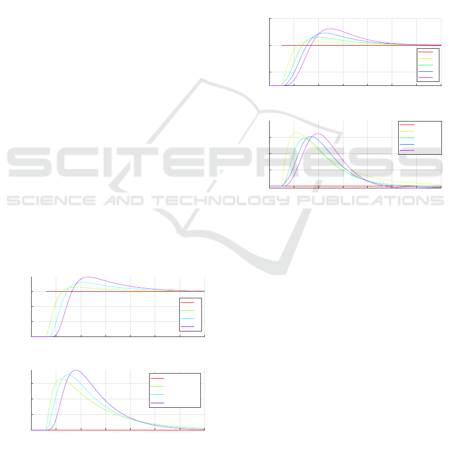
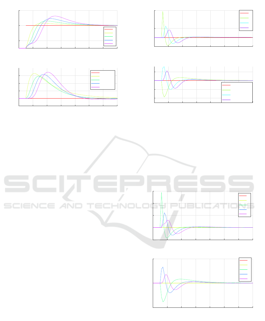
4.1 Leading Vehicle Changing Velocity
Scenario
Several vehicles are set up, with the leading vehi-
cle i = 0 accelerating from 15 m/s to 18 m/s instantly.
This scenario mimics a step-input disturbance to the
following vehicles. The controller should adapt to the
new velocity and drive back the distance headway to
its desired level, i.e., 20 m.
4.1.1 MOTIF1 Closed-Loop Simulation
In this simulation scenario, the first vehicle is mod-
eled as a step-input signal. All other vehicles are
modeled using MOTIF1. Therefore, they only take
into account the vehicle directly ahead. The vehicles
can follow the desired speed defined by the leading
vehicle. At the same time, the controller drives the
headway distance to its desired level. In this MOTIF
configuration, the vehicle starts compensating for the
deviation in states only when the preceding vehicle
starts responding.
0 1 2 3 4 5 6 7
Time [s]
15
16
17
18
Velocity [m/s]
Velocity
0
1
2
3
0 1 2 3 4 5 6 7
Time [s]
20
20.2
20.4
20.6
Headway [m]
Headyway Distance
Reference
1
2
3
Figure 4: MOTIF1 closed loop simulation of leading vehi-
cle changing velocity scenario.
4.1.2 MOTIF2 Closed Loop Simulation
In this simulation scenario, five vehicles exist. The
first vehicle is modeled as a step-input signal. The
second vehicle is modeled using OVM with MOTIF1
since MOTIF2 is not defined for it. The rest of the ve-
hicles are modeled using the optimal velocity model
of MOTIF2. The steady state of this configuration
is identical to Section 4.1.1. However, the transient
response takes place earlier as per the imposed MO-
TIF configuration. Higher velocity overshoots are ob-
served and less headway distance overshoots than in
Section 4.1.1.
0 1 2 3 4 5 6 7
Time [s]
16
18
20
Velocity [m/s]
Velocity
0
1
2
3
4
0 1 2 3 4 5 6 7
Time [s]
20
20.2
20.4
20.6
Headway [m]
Headyway Distance
Reference
1
2
3
4
Figure 5: MOTIF2 closed loop simulation of leading vehi-
cle changing velocity scenario.
4.1.3 MOTIFn Closed Loop Simulation
In this simulation scenario, 5 vehicles are instantiated.
Each vehicle’s MOTIF equals its i subscript; for ex-
ample, the vehicle with i = 1 is MOTIF1, and the ve-
hicle with i = 2 is MOTIF2, and so on. This config-
uration allows each vehicle to obtain the velocity of
each preceding and leading vehicle. In Figure 6, the
vehicles start responding by increasing their veloci-
ties at the exact time point when the leading vehicle
changes its velocity. This MOTIF configuration has
the highest overshoot in both velocity and headway,
this happens because the controller does not discrim-
inate between disturbances signals i.e ˜v
i−1
and ˜v
i−m
and the integral gains are the same for all vehicles.
More careful selection of the integral gain reduces the
overshoot.
In the MOTIFn configuration, the responsiveness
for perpetuation is simultaneous in which the follow-
Optimal Velocity Model Based CACC Controller for Urban Scenarios
333

0 1 2 3 4 5 6 7
Time [s]
16
18
20
Velocity [m/s]
Velocity
0
1
2
3
4
0 1 2 3 4 5 6 7
Time [s]
19.8
20
20.2
20.4
20.6
Headway [m]
Headyway Distance
Reference
1
2
3
4
Figure 6: MOTIFn closed loop simulation of leading vehi-
cle changing velocity scenario.
ing vehicles start responding at the time instance of
perpetuation occurring which is a significant advan-
tage over other CACC systems where they respond
asynchronously as in (Bekiaris-Liberis, 2023), (Chen
et al., 2024) (Xing et al., 2022) and others. By im-
plementing a comprehensive assessment mechanism,
we can pinpoint and address the vulnerabilities in our
CACC. This targeted approach will enable us to en-
hance the overall resilience and responsiveness of our
transportation system by making vulnerable vehicle
central in the information flow and the other vehicles
respond to the vulnerable vehicles simultaneously.
In all simulation scenarios of different MOTIFs,
the controller is able to keep the desired headway even
when the dynamics are different.
4.2 Velocity Disturbance Scenario
Several vehicles are set up, a non-leading vehicle ve-
locity is injected with a velocity disturbance. This al-
lows us to inspect the controller on the vehicle level
and on the following vehicles. This scenario mimics
an impulse input to the vehicle and an impulse distur-
bance on the following vehicles.
4.2.1 MOTIF1 Closed Loop Simulation
Figure 7 shows the states’ evolution of three MOTIF1
vehicles. An impulse occurs in vehicle 1. The vehicle
states return to the desired state with an overshoot in
the headway value. The following vehicles also return
to the desired states.
0 1 2 3 4 5 6 7
Time [s]
14
16
18
Velocity [m/s]
Velocity
0
1
2
3
0 1 2 3 4 5 6 7
Time [s]
19.6
19.8
20
20.2
Headway [m]
Headyway Distance
Reference
1
2
3
Figure 7: MOTIF1 closed loop simulation of leading vehi-
cle 1 velocity disturbance scenario.
4.2.2 MOTIF2 Closed Loop Simulation
In this simulation, vehicle 1 is MOTIF1, and the fol-
lowing vehicles are MOTIF2. An impulse occurs in
vehicle 2. The vehicle returns to the desired state. 8.
The following vehicles of vehicle 2 start responding
to impulse at the same time.
0 1 2 3 4 5 6 7
Time [s]
14
15
16
17
18
Velocity [m/s]
Velocity
0
1
2
3
4
0 1 2 3 4 5 6 7
Time [s]
19.5
20
20.5
Headway [m]
Headyway Distance
0
1
2
3
4
Figure 8: MOTIF2 closed loop simulation of leading vehi-
cle changing velocity scenario.
In both cases subsections 4.2.1 and 4.2.2 the con-
troller deals with the disturbance without showing
signal propagation in either velocity or headway from
leading to following vehicles.
VEHITS 2024 - 10th International Conference on Vehicle Technology and Intelligent Transport Systems
334

5 CONCLUSION
In this work, a new CACC system that exhibits the
Optimal Velocity Model has been introduced. The
new CACC system uses the adopted MOTIF concept
to define the system dynamics. The linearized dy-
namic equations have been derived for any MOTIF.
Several Linear Quadratic Controllers have been in-
cluded. The main focus was on LQR with integral
action. Simulations of different MOTIFs were pre-
sented. The LQR with the integral action controller is
able to bring the system states to the desired value and
is indifferent to the MOTIF. In this work, the internal
dynamics of the vehicles were ignored. Inclusion of
longitudinal dynamics as a first-order linear system
is a potential future work. From an vehicle perspec-
tive, the LQR with integral action performs very well;
however, from a multiple-vehicles perspective, it is
clear that wave propagation through vehicles takes
place, this happens as a result of the integral part of
the controller. This limitation is very significant and
needs to be addressed in further future work.
REFERENCES
˚
Astr
¨
om, K. J. and Murray, R. M. (2021). Feedback systems:
an introduction for scientists and engineers. Princeton
university press.
Bando, M., Hasebe, K., Nakayama, A., Shibata, A., and
Sugiyama, Y. (1994). Structure stability of congestion
in traffic dynamics. Japan Journal of Industrial and
Applied Mathematics, 11(2):203–223.
Bando, M., Hasebe, K., Nakayama, A., Shibata, A., and
Sugiyama, Y. (1995). Dynamical model of traffic con-
gestion and numerical simulation. Physical review E,
51(2):1035.
Bekiaris-Liberis, N. (2023). Robust String Stability and
Safety of CTH Predictor-Feedback CACC. IEEE
Trans. Intell. Transp. Syst., 24(8):8209–8221.
Bellman, R. (1966). Dynamic programming. Science,
153(3731):34–37.
Brand, C., Anable, J., and Morton, C. (2019). Lifestyle,
efficiency and limits: modelling transport energy and
emissions using a socio-technical approach. Energy
Efficiency, 12(1):187–207.
Chen, D., Zhang, K., Wang, Y., Yin, X., Li, Z., and Filev, D.
(2024). Communication-efficient decentralized multi-
agent reinforcement learning for cooperative adaptive
cruise control. IEEE Transactions on Intelligent Vehi-
cles.
Fu, A., Chen, S., Qiao, J., and Yu, C. (2023). Peri-
odic Event-Triggered CACC and Communication Co-
design for Vehicle Platooning. ACM Trans. Cyber-
Phys. Syst., 7(4):1–19.
Ge, J. I. and Orosz, G. (2016). Optimal Control of Con-
nected Vehicle Systems With Communication Delay
and Driver Reaction Time. IEEE Trans. Intell. Transp.
Syst., 18(8):2056–2070.
Hsueh, K.-F., Farnood, A., Al-Darabsah, I., Al Saaideh, M.,
Al Janaideh, M., and Kundur, D. (2022). A Deep Time
Delay Filter for Cooperative Adaptive Cruise Control.
ACM Trans. Cyber-Phys. Syst.
Liu, J., Zhou, Y., and Liu, L. (2023). Communication
delay-aware cooperative adaptive cruise control with
dynamic network topologies-a convergence of com-
munication and control. Digital Communications and
Networks.
Malkapure, H. G. and Chidambaram, M. (2014). Compar-
ison of two methods of incorporating an integral ac-
tion in linear quadratic regulator. IFAC Proceedings
Volumes, 47(1):55–61.
Naidu, D. S. (2002). Optimal control systems. CRC press.
Nguyen, T.-A. and Bestle, D. (2007). Application of opti-
mization methods to controller design for active sus-
pensions. Mechanics based design of structures and
machines, 35(3):291–318.
Pontryagin, L. S. (1987). Mathematical theory of optimal
processes. CRC press.
Reimann, M. (2008). Simulationsmodelle im Verkehr. ht
tps://docplayer.org/39907139-Simulationsmodelle-i
m-verkehr.html. [Online; Sep, 2022].
Scokaert, P. O. and Rawlings, J. B. (1998). Constrained
linear quadratic regulation. IEEE Transactions on au-
tomatic control, 43(8):1163–1169.
Shladover, S. E., Nowakowski, C., Lu, X.-Y., and Ferlis,
R. (2015). Cooperative adaptive cruise control: Def-
initions and operating concepts. Transportation Re-
search Record, 2489(1):145–152.
Wang, Z., Wu, G., and Barth, M. J. A Review on Cooper-
ative Adaptive Cruise Control (CACC) Systems: Ar-
chitectures, Controls, and Applications. In 2018 21st
International Conference on Intelligent Transporta-
tion Systems (ITSC), pages 04–07. IEEE.
Xing, H., Ploeg, J., and Nijmeijer, H. (2022). Robust CACC
in the Presence of Uncertain Delays. IEEE Trans. Veh.
Technol., 71(4):3507–3518.
Yang, T., Murguia, C., Ne
ˇ
si
´
c, D., and Lv, C. (2023). A
Robust CACC Scheme Against Cyberattacks via Mul-
tiple Vehicle-to-Vehicle Networks. IEEE Trans. Veh.
Technol., 72(9):11184–11195.
Zhang, L. and Orosz, G. (2013). Designing network motifs
in connected vehicle systems: delay effects and sta-
bility. In Dynamic Systems and Control Conference,
volume 56147, page V003T42A006. American Soci-
ety of Mechanical Engineers.
Zhang, L. and Orosz, G. (2015). Connected vehicle sys-
tems with nonlinear dynamics and time delays. IFAC-
PapersOnLine, 48(12):370–375.
Zhongwei, F., Qin, K., Jiao, X., Du, F., and Li, D. Co-
operative Adaptive Cruise Control for Vehicles Under
False Data Injection Attacks. In 2023 IEEE 6th In-
ternational Conference on Industrial Cyber-Physical
Systems (ICPS), pages 08–11. IEEE.
Optimal Velocity Model Based CACC Controller for Urban Scenarios
335