Outlier Detection Through Connectivity-Based Outlier Factor for

Software Defect Prediction

Andrada-Mihaela-Nicoleta Moldovan

and Andreea Vescan

Computer Science Department, Faculty of Mathematics and Computer Science,

Babes¸-Bolyai University, Cluj-Napoca, Romania

Keywords:

Outlier Detection, Anomaly Detection, Software Defect Prediction.

Abstract:

Regression testing becomes expensive in terms of time when changes are often made. In order to simplify

testing, supervised/unsupervised binary classiﬁcation Software Defect Prediction (SDP) techniques may rule

out non-defective components or highlight those components that are most prone to defects. In this paper,

outlier detection methods for SDP are investigated. The novelty of this approach is that it was not previously

used for this particular task. Two approaches are implemented, namely, simple use of the local outlier factor

based on connectivity (Connectivity-based Outlier Factor, COF), respectively, improving it by the Pareto rule

(which means that we consider samples with the 20% highest outlier score resulting from the algorithm as

outliers), COF + Pareto. The solutions were evaluated in 12 projects from NASA and PROMISE datasets.

The results obtained are comparable to state-of-the-art solutions, for some projects, the results range from

acceptable to good, compared to the results of other studies.

1 INTRODUCTION

Software testing is a highly integrated and equally im-

portant step in software development as the building

itself (Khan and Khan, 2014). Because the costs of

testing are both ﬁnancially and time-consuming, any

tool that may autonomously rule out from testing a

majority of components that are highly unlikely to

contain defects or point out the few that are highly

prone to defects is useful in reducing both invested

time and the price of testing.

There are a few approaches for determining bugs

in software systems, one of which is manual testing,

which includes acceptance testing, integration testing,

and regression testing (Myers et al., 2011). However,

these processes require testers that perform explicit

instructions at given times, for example, acceptance

testing involves testing the whole software system af-

ter a major release.

In order to simplify this activity, automatic testing

is used to automatically run test cases, but exploratory

testing, that is, testers explore the application from

different perspectives to identify corner cases, is still

not replaceable by automation software. Another case

in which automatic testing is not useful is in early

https://orcid.org/0009-0006-6289-9869

https://orcid.org/0000-0002-9049-5726

stage testing, as the application is still in the early

stages.

Software defect prediction may not only simplify

exploratory and early-stage testing by telling testers

which components are most prone to defects but also

automatic testing by identifying those parts of the ap-

plication that require more attention. There are mul-

tiple approaches to the problem: supervised (Afric

et al., 2020), unsupervised or semi-supervised meth-

ods (Wang et al., 2016). After investigating exist-

ing research that proposes to correlate defective mod-

ules with outliers with promising results for unsu-

pervised techniques such as Isolation Forest (Ding,

2021) (Ding and Xing, 2020) or SVMs (Moussa et al.,

2022), we have decided to investigate similar ap-

proaches.

Thus, various reasons motivate the current study.

The primary motivation and the initial idea was to

identify an Outlier Detection (OD) that has not yet

been used for the SDP task. Studying the current liter-

ature regarding the problem (e.g., (Afric et al., 2020),

(Dimitrov and Zhou, 2009), etc.), it has become ob-

vious that the anomaly detection approach is suitable

for it; however, we have discovered that most studies

focus on a limited number of methods, leaving a few

others with undocumented results.

The initial approach was to collect as many OD

474

Moldovan, A. and Vescan, A.

Outlier Detection Through Connectivity-Based Outlier Factor for Software Defect Prediction.

DOI: 10.5220/0012683400003687

Paper published under CC license (CC BY-NC-ND 4.0)

In Proceedings of the 19th International Conference on Evaluation of Novel Approaches to Software Engineering (ENASE 2024), pages 474-483

ISBN: 978-989-758-696-5; ISSN: 2184-4895

methods as possible, ﬁlter out those that had already

been documented by other studies, then perform tests

on the remaining ones, in the hope of obtaining simi-

lar results to those that have already been successfully

used for the task, namely Isolation Forest (Ding et al.,

2019), (Ding and Xing, 2020), SVM (Moussa et al.,

2022).

One of the objectives of the paper is to identify the

existing OD techniques for SDP. After gathering all

the OD methods that have not yet been experimented

with for the SDP (Software Defect Prediction) task,

the intuition is that some of them may possess a few

qualities, such as working well with sparse datasets

but also being scalable, simple to implement, gener-

alizable or even particularly great for our problem.

The second aim of the paper is to investigate the

discovered OD in the context of SDP. Afterward, we

want to identify the best performing ones and doc-

ument the results, examine different data processing

techniques, and experiment with possible enhance-

ments to the methods.

The contributions in this paper are composed of

performing a Systematic Literature Review in the

context of Software Defect Prediction using Outlier

Detection, implementing the model for Connectivity-

based Outlier Factor following the algorithm from the

original paper presenting it (Tang et al., 2002), apply-

ing it to Software Defect Prediction datasets, enhanc-

ing the method with an additional approach follow-

ing the Pareto Rule, and presenting some results and

conclusions regarding the previous steps. Most im-

portantly, the results of this particular solution, that

is, connectivity-based outlier detection (Tang et al.,

2002) have never been discussed before in the context

of Software Defect Prediction.

The work is organized as follows: in Section 2 we

present background concepts on the subject of Soft-

ware Defect Prediction and Outlier Detection and re-

view the current state of the art in the context of SDP,

Section 3 brieﬂy describes our proposed approach,

presenting the COF and COR+Pareto approach along

with the dataset used, while Section 4 reports the ex-

periments carried out on our models together with an

analysis of the results. Section 5 outlines the threats

to validity, while Section 6 states the conclusions and

future work.

2 BACKGROUND AND RELATED

WORK

In this section, we present the concepts used in this

paper, namely software defect prediction and outlier

detection, along with research studies on OD for SDP.

2.1 Software Defect Prediction

Software defect prediction is the solution to the task

of identifying potential issues in modules, classes, or

methods before their occurrence. With the help of

datasets that store attributes that deﬁne the complex-

ity, size, or number of collaborators of the code, the

aim is to determine whether an instance is potentially

faulty.

A typical approach to SDP implies the following

steps: data collection - documenting historical infor-

mation regarding bugs or changes, feature selection

- ﬁltering the most relevant attributes, model training

- creating statistical or machine learning methods to

build a predictive tool for the task, and model assess-

ment - cross-validation or comparison of results with

correctly labeled instances.

2.2 Outlier Detection

Outlier Detection (OD), also referred to as Anomaly

Detection, is a technique to identify samples from a

crowd that deviate from the average, to compare and

take noisy data from statistics. Data points known as

outliers deviate considerably from other observations

in a dataset and may hint at anomalous behavior, mis-

takes, or intriguing patterns.

There are various methods to ﬁnd outliers (Han

et al., 2022), including Statistical Methods, Distance-

Based Methods, Density-Based Methods, Clustering-

Based Methods, and Machine Learning-Based Meth-

ods.

Most of the research on software fault prediction

employs supervised classiﬁcation techniques (Wa-

hono, 2015), which can be time consuming due to

training and the collection of large amounts of labeled

training data. To reduce the need for labeled data,

unsupervised defect prediction models often employ

clustering techniques; nevertheless, identifying clus-

ters as defective is a difﬁcult task (Moshtari et al.,

2020).

2.3 Related Work on SDP and OD

A rigorous and thorough strategy for locating, as-

sessing, and synthesizing current research related to

a particular research question or topic is a System-

atic Literature Review presented by Kitchenham et

al. in (Kitchenham and Charters, 2007). It involves

doing a thorough search for pertinent databases and

other sources, followed by a methodical evaluation

and analysis of the studies that have been found.

The steps of the conducted SLR are respected and

exempliﬁed in the Master’s Thesis (Moldovan, 2023).

Outlier Detection Through Connectivity-Based Outlier Factor for Software Defect Prediction

475

In this paper, only the synthesis is presented due to

page limitation and because the aim of the paper is to

investigate on outlier detection for SDP.

We compile and evaluate previous work on source

code defect prediction utilizing anomaly detection

approaches for our research article by conducting a

comprehensive literature review. In what follows,

we outline the ﬁndings regarding outlier detection for

predicting software defects, categorizing the research

studies into 4 major groups. The assumption that

software problems should be considered anomalies is

supported by a number of research studies, more of

which are released every year. Most of these stud-

ies compare the results of the technique with those

of other common classiﬁers. As a topic in the ﬁeld

of Software Engineering, Software Defect Prediction

has been granted signiﬁcant interest, and with con-

siderable research came the Anomaly Detection ap-

proach that can be done by using either machine

learning or statistical methods.

2.4 Machine Learning Approach to

Anomaly Detection for SDP

The use of machine learning techniques is one of

the key strategies for the detection of anomalies for

the prediction of software faults. Numerous re-

search studies have investigated the use of various

machine learning techniques, such as k-nearest neigh-

bors (Moshtari et al., 2020). These algorithms are

trained on historical data to discover patterns of soft-

ware ﬂaws and spot unusual behavior that could point

to the possibility of errors in the future.

The authors in the research paper (Ding et al.,

2019) propose a new approach to SDP using isola-

tion forest, an unsupervised machine learning algo-

rithm for anomaly detection. The proposed method

involves ﬁrst extracting features from software met-

rics and then using an isolation forest to identify po-

tentially anomalous instances in the feature space.

The performance of the method is evaluated on sev-

eral datasets and compared with other state-of-the-art

methods such as support vector machines and deci-

sion trees (Agrawal and Menzies, 2018).

Another anomaly detection method that was found

to be suitable for the SDP task is (Moussa et al.,

2022) which uses a support vector machine (SVM).

The study focuses on comparing the performance of

OCSVM with traditional classiﬁcation models such

as decision trees and logistic regression and inves-

tigates the impact of different hyperparameters on

the performance of OCSVM. The results suggest that

OCSVM does not outperform the Two-class SVM,

which remains highly successful for the task.

2.5 Statistical Machine Learning

Methods Approach to Anomaly

Detection for SDP

Using statistical approaches is another way to ad-

dress the same task. These techniques look at the

distribution of software metrics for abnormalities that

could point to ﬂaws. Regression analysis (Neela et al.,

2017) is one popular statistical technique for ﬁnding

anomalies, just as correlation analysis (Zhang et al.,

2022), and hypothesis testing (Dimitrov and Zhou,

2009).

The use of ensemble approaches for anomaly de-

tection in software defect prediction has also been ex-

amined in a number of research studies (Zhang et al.,

2022), (Ding and Xing, 2020). To increase the preci-

sion and resilience of the anomaly detection process,

ensemble approaches mix a variety of machine learn-

ing algorithms or statistical techniques.

In (Afric et al., 2020) a novel statistical approach

is proposed to predict software defects by treating the

problem as an anomaly detection task in which indi-

vidual and collective outliers are considered. The au-

thors argue that existing defect prediction techniques

suffer from various limitations, such as the need for

labeled data and the inability to handle complex code

patterns. To address these issues, they present a

new method that uses unsupervised anomaly detec-

tion techniques to identify code ﬁles that deviate sig-

niﬁcantly from normal patterns and are likely to con-

tain defects.

The method suggested by Neela et al. (Neela

et al., 2017) involves ﬁnding possibly anomalous in-

stances in the feature space using unsupervised ma-

chine learning methods such as principal component

analysis and isolation forest. It is compared to other

cutting-edge software defect prediction techniques

like (Menzies et al., 2006), the average balance be-

ing around 63% for the univariate model and 69% for

the multivariate model, respectively, compared to the

average accepted norm that is set at about 60% ac-

cording to (Menzies et al., 2006).

In (Ding and Xing, 2020), they propose an im-

proved ensemble approach for SDP using pruned

histogram-based isolation forest (PHIF), a variant of

the isolation forest algorithm that uses histograms to

accelerate the tree-building process. The proposed

approach involves using PHIF to identify potentially

anomalous instances in the feature space and then us-

ing a decision tree to classify the instances as defec-

tive or non-defective. The performance of the ap-

proach is evaluated on several datasets and compared

to another state-of-the-art method used for debugging

that is based on failure-inducing (Gupta et al., 2005).

ENASE 2024 - 19th International Conference on Evaluation of Novel Approaches to Software Engineering

476

3 OUR RESEARCH PROPOSAL

ON SDP USING OD

This section aims to deﬁne and present the method-

ologies and aggregation tools that have been used in

the process of creating this study together with its ap-

plication.

3.1 From LOF to Connectivity-Based

LOF

We describe the Connectivity-based Outlier Factor

(COF) (Tang et al., 2002) by starting with the orig-

inal algorithm, the Local Outlier Factor (LOF). We

introduce the LOF, display and explain the involved

formulas, then deﬁne the enhancements brought to it

to create the COF. Information about the implemented

approaches is provided at this ﬁgshare link (Moldovan

and Vescan, 2023).

To understand the algorithm, we must ﬁrst under-

stand how LOF works: Let k, p and o ∈ D, where

D ⊂ N, then the distance between o and its k-th near-

est neighbor can be written as k − distance (p). Let

us also deﬁne the N

k−distance

(p)

, which contains a col-

lection of distances from a data point to its k-nearest

neighbors.

Another term that needs to be introduced is the

reachability distance between p (as observation point)

and k:

reach−disk

(p, o) = max{k-distance (o), dist(p, o)}.

Furthermore, we may introduce the local reach-

ability for the distance /empthk (as in (Tang et al.,

2002) ), having p as the center of observation is de-

ﬁned as follows:

lrd

(p) =

∑

o∈N

k−distance

(p)

reach dist

(p,o)

k−distance(p)

(p)

−1

In other words, we may deﬁne the local reacha-

bility distance (lrd) as an inverted avg. distance be-

tween the observation point p p and instances stand-

ing in its k-neighborhood, making the local density

another term for the lrd. Finally, we get the LOF for-

mula which is:

LOF

(p) =

∑

o∈N

k−distance

(p)

lrd

(o)

lrd

(p)

k−distance(p)

(p)

As presented by the formula and mentioned by

Breunig et al. (Breunig et al., 2000), p’s density is

inversely proportional to its LOF, meaning that a high

density indicates a lower chance of a point being an

outlier and vice versa. Obviously, there is still room

for interpretation of the threshold value that deﬁnes at

exactly what distance a point is or is not labeled as an

outlier, which is best determined by the user depend-

ing on the particular problem.

For understanding, the authors of (Tang et al.,

2002) have shown that there are some cases that can-

not be handled simply by the LOF algorithm because

its ﬂaw lies in not differentiating low density from

isolativity. That being said, it is possible to have out-

liers of a group of entities, but for the outliers not to

be outside of the k-distance for all of the points, and

the proof can be found (Tang et al., 2002). The prob-

lem is that there is a threshold for k, such that it is

set lower; the formula will not be relevant for den-

sity group C2 and they will all be labeled as outliers,

while if setting k is higher, then it will not label o1

as an outlier anymore as the distance between o1 and

density group C1 is lower than the distance from any

actual neighbors of density group C2.

3.2 Connectivity-Based Outlier Factor

(COF)

To solve the problem of separating “isolativity” from

“low density”, Breunig et. al (Breunig et al., 2000)

wanted to reformulate the deﬁnition of local density

such that an outlier will not only be labeled so based

on pure distance from its closest neighbor, but also

consider the shape of close neighborhoods to evalu-

ate whether it ﬁts into it. Therefore, isolation points

out a sample with low density, but it is not true the

other way around. In most cases, departing from a

linked pattern produces an isolated outlier, whereas

diverging from a high-density pattern produces a low-

density outlier. Both situations should be taken into

account by an outlier indicator.

The average distance of consecutive points in a

neighborhood of point

p, as well as the average of avg

(the distance of consecutive points between point p’s

k-distance neighbors and their own k-distance neigh-

bors), constitute the connectivity-based outlier factor

in p. Displays how much a point departs from a pat-

tern.

The full deﬁnition may be found in the original pa-

per, but we will brieﬂy present the equation describing

the formula of the connectivity-based outlier factor of

a point p ∈ D:

COF

(p) =

(p)

·ac−dist

(p)

∑

o∈N

(p)

ac−dist

(o)

where N

(p) is the set of k-nearest neighbors of p.

The ac-dist denotes the average chained distance (as

provided in (Tang et al., 2002)) and is computed by

the following formula:

Outlier Detection Through Connectivity-Based Outlier Factor for Software Defect Prediction

477

ac − dist

) =

r−1

∑

r−1

i=1

2(r−i)

· dist (e

where s =

⟨

, p

, . . . , p

⟩

is an SBN-

path. A set-based nearest chain, or SBN-

chain, w.r.t. s is a sequence

⟨

, . . . , e

r−1

⟩

s.t. ∀ 1 ≤ i ≤ r − 1, e

= (o

, p

i+1

) where

∈

{

, . . . , p

}

, and dist(e

) = dist (o

, p

i+1

) =

dist(

{

, . . . , p

}

{

i+1

, . . . , p

}

). We call each e

edge and the sequence

⟨

dist(e

), . . . , dist(e

r−1

)

⟩

the

cost description of

⟨

, . . . , e

r−1

⟩

3.3 COF Implementation

To implement the algorithm presented in the previous

section, we started from the implementation proposed

by Songqiao (Han et al., 2022) that can be accessed

through the PyOD library in Python. Because there

was room for improvement towards simplicity in their

code, we have rewritten the model in order to use it

outside of their library and still follow the approach

introduced by Tang (Tang et al., 2002).

Han et al. (Han et al., 2022) have identiﬁed the

largest possible set of OD methods, documenting re-

sults for all kinds of tasks that could be addressed with

the approaches, but missing out on the problem of

SDP. Therefore, our study comes as an additional im-

provement to their work: we have rewritten the model

in a simple manner and evaluated it on multiple SDP

datasets from two different repositories.

An explanation of the model is available in the

code listed on the ﬁgshare link (Moldovan and Ves-

can, 2023). Similarly to the SLR, a full description

of the algorithm may be found in the master’s thesis

(Moldovan, 2023), where we have elaborated on the

steps, methods, and origins of the resources involved

in the application.

3.4 SDP Datasets

For designing, running and evaluating the experi-

ments, different datasets that are commonly used for

software defect prediction were used.

We have evaluated the projects on datasets from

the following repositories: NASA MDP, Apache

Log4J and Apache ANT, CAMEL, and IVY. More

precisely, we have successfully obtained notable re-

sults (as provided in the next sections) by running the

model with the following ﬁles in .csv format: cm1,

jm1, kc1, pc1, ant-1.3, ant-1.4, ant-1.5, ant-1.6, ant-

1.7, log4j-1.0, log4j-1.1, log4j-1.2, camel-1.0, camel-

1.2, camel-1.4, camel-1.6, ivy-1.1, ivy-1.4, ivy-2.0.

It is worth mentioning that CM1 is a dataset ex-

tracted from the application version 3.2 of the soft-

ware project “CruiseControl”, JM1 is derived from

the application version 3.4 of the software project

“Jedit”, while KC1, and PC1 deﬁne the application

versions 2.0 and 3.0 of the software project “KC1”

(Kemerer and Porter) developed at NASA. For the

rest of the datasets, multiple versions have been uti-

lized and are mentioned within the rows of the ta-

ble. More information regarding datasets descrip-

tion can be found in the Master’s Thesis (Moldovan,

2023). While we have indeed amassed validation re-

sults for the application of the algorithm on the ANT

and LOG4j datasets, our objective was to juxtapose

these ﬁndings with established metrics found in the

existing literature, which exclusively displays results

assessed on the NASA datasets.

Table 1 contains information about the projects

with columns representing: F (Features), M (Mod-

ules), D (Defects), %D (% Defects), and C (Corpus).

Table 1: List of selected datasets.

Dataset

Name

F M D %D C

CM1 39 344 42 13,91 NASA

KC1 39 2096 325 15.51 NASA

JM1 23 9593 1759 18,34 NASA

PC1 39 759 61 8.04 NASA

Ant-1.3 24 125 20 16.00 PROMISE

Ant-1.4 24 178 40 22.47 PROMISE

Ant-1.5 24 293 32 10.92 PROMISE

Ant-1.6 24 351 92 26.21 PROMISE

Ant-1.7 24 745 166 22.28 PROMISE

Log4j-1.0 24 135 34 25.19 PROMISE

Log4j-1.1 24 109 37 33.95 PROMISE

Log4j-1.2 24 205 189 92.2 PROMISE

3.5 The Pareto Principle Approach

Moshtari et al. (Moshtari et al., 2020) have proposed

a distinctive approach to make use of a binary clas-

siﬁer, which presented impressive results considering

its simplicity.

The Pareto principle, informally known as the

80/20 rule, claims that 80% of the results are the out-

comes of 20% of the causes, an observation made in

1906 by economist Vilfredo Pareto who noticed that

80% of the land is owned by 20% of the population.

Therefore, applying the rule to our subject, we get

the hypothesis that 20% of the modules contain 80%

of the defects. Combining this with our initial hypoth-

esis, which states that the defective modules have dif-

ferent characteristics compared to the non-defective

ones, hence having higher chances of being outliers,

we may build a new technique for identifying them.

However, before applying an approach that fol-

lows the hypothesis, we must ﬁrst assess that one is

ENASE 2024 - 19th International Conference on Evaluation of Novel Approaches to Software Engineering

478

true by verifying the proportion of defective instances

from our datasets. Following Table 1 of datasets and

calculating the mean average of all instances from the

column Defects%, we get a value of 24.5, supporting

the hypothesis. Additionally, the approach is proved

to be efﬁcient in the context of SDP by Moshtari et al.

(Moshtari et al., 2020).

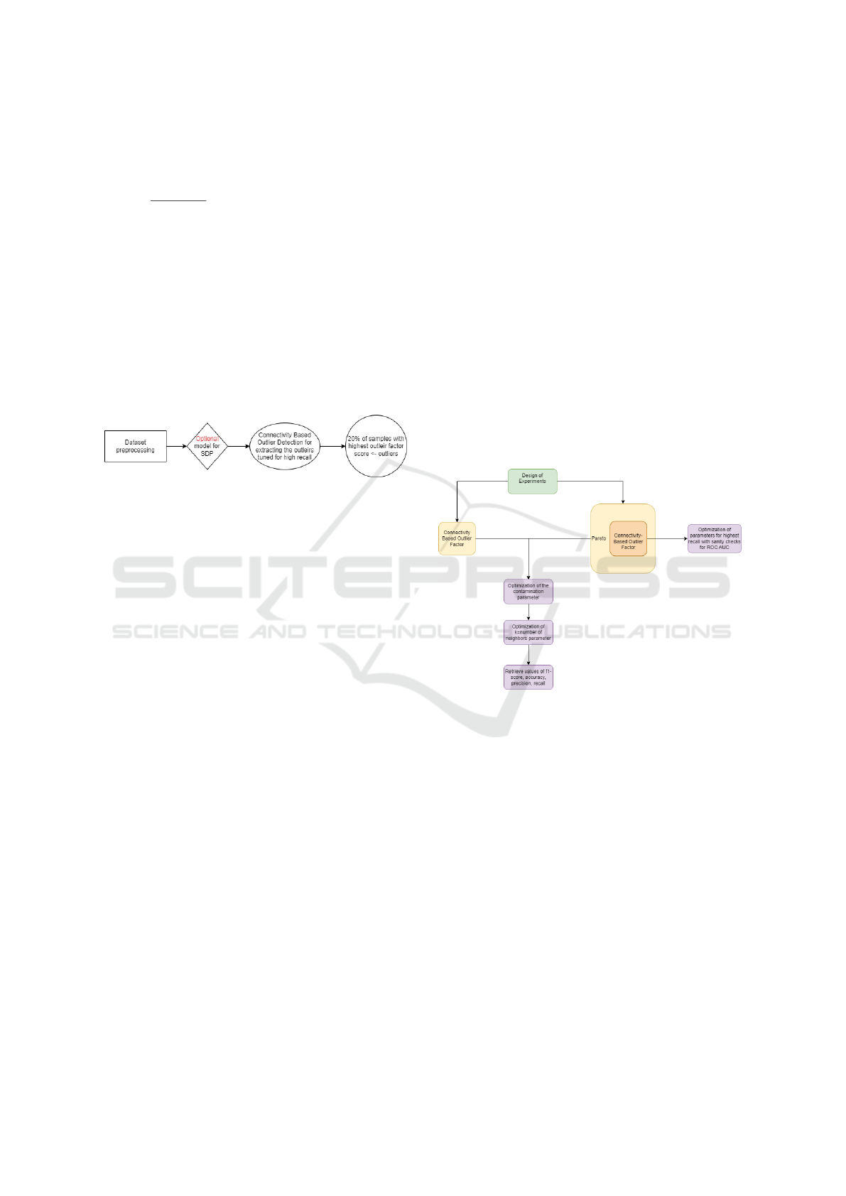
Furthermore, we may deﬁne the following method

(see Figure 1): tune our classiﬁer so that it supports

the highest possible recall, while only focusing on

performing sanity checks for the other metrics. A

high recall value is desired because programmers can

ﬁnd most of the ﬂaws (that 20% “vital” issues) with a

simple method based on outlier detection. Afterward,

ascending sort the resulting array from the classiﬁer

and extract exactly the last 20% that we label as “de-

fective”.

Figure 1: Proposed approach leveraging the Pareto princi-

ple.

3.6 Feature Selection, Feature Scaling

Multiple experiments with various numbers of fea-

tures were performed with the aim of determining

which number of features is ideal, as well as how

to scale them for the best results. For this step, the

datasets from NASA i.e., cm1, kc1, jm1, and pc1 were

used. The conclusion is that the algorithm’s effective-

ness is anyhow not affected by the number of selected

features and their scaling nevertheless.

The results of the execution where we have passed

between k=5 and k=10 number of features outlined

that none of these numbers of selected features lead

to notably different results, which similarly has been

the case for the implication of MinMaxScaler from

Sklearn (Kramer and Kramer, 2016).

A theory about the lack of importance in feature

selection and normalization for COF is that the fea-

tures ﬁlter and sort themselves in the algorithm, de-

pending on their distances and outlier factors.

4 EXPERIEMENTS AND

RESULTS

This section outlines the design of the experiments

along with the metrics used for the evaluation. In the

second part, the results are provided and discussed.

4.1 Design of Experiments

In order to evaluate the potential real-life use of the

method in the context of SDP, two main approaches

have been considered. First, the basic COF is applied

to the algorithm, and second, the enhancement of the

COF by applying the Pareto principle (Moshtari et al.,

2020), COF+Pareto.

The two views of the experiments are shown in

Figure 2. Two parameters, namely contamination

(i.e., the threshold value for an instance that is consid-

ered an outlier, meaning that if contamination is 3.1,

any value equal to or higher than it will be an out-

lier) and the number of neighbors (i.e., the k value,

as required in the KNN algorithm (Moshtari et al.,

2020)), are optimized for both approaches. Addition-

ally, for the second approach, we focus on an 80%

recall, which means that we aim for this value while

maintaining the ROC AUC under a sanity check, as it

reﬂects the overall success of the classiﬁer.

Figure 2: Design of experiments.

4.2 Evaluation Approach and Metrics

The steps of experimental evaluation are provided, fo-

cusing on each element of the methodology and the

metrics used.

4.2.1 Cross-Validation

Cross-validation (Berrar, 2019) is a trusted and reli-

able method for assessing machine learning perfor-

mance, providing information on model overﬁtting,

underﬁtting, or failing to generalize a pattern. We

evaluated the f-measure using this method and chose

k=5 for the number of folds presented in Figure 3.

While utilization of K-fold cross-validation is preva-

lent within learning-based algorithms, involving the

division of the dataset into k subsets for iterative as-

signment as either training or validation subsets, its

Outlier Detection Through Connectivity-Based Outlier Factor for Software Defect Prediction

479

application extends beyond. We have adapted this

methodological framework to our non-learning algo-

rithm, employing it to gauge its generalization capac-

ity towards new data points.

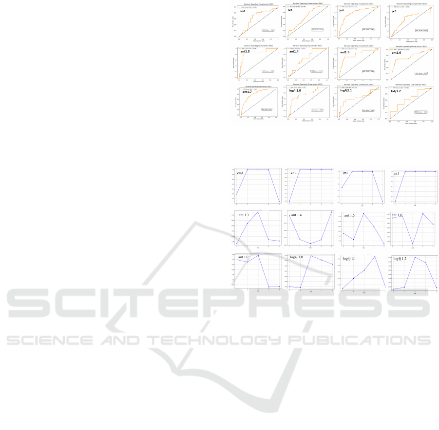
We may notice from the cross-validation scores 3

that running the experiments on the NASA datasets

(e.g. CM1, KC1, JM1, and PC1) F1 values equal to

1.0 are attained in 3/5 folds, namely 2, 3, and 4. The

rest of the experiments only reach values of up to 0.75

for exclusively a single point. A possible correlation

between the number of samples in a dataset and the

F-mean values may be considered, by observing that

the scores attained for each dataset are directly pro-

portional to the number of instances: cm1 dataset -

488 samples, kc1 dataset - 2109 samples, jm1 dataset

- 521 samples, ant1.7 dataset - 744 samples. In con-

trast to the high values for large datasets, there is a

maximum score of 0.24 for the log4j 1.2 dataset, con-

sisting of only 200 instances.

4.2.2 The Sanity Checks

Sanity checking (Doshi-Velez and Perlis, 2019) is

responsible for assessing the performance of a cer-

tain ML model, ensuring that the results have passed

a threshold normally deﬁned as “random guessing”.

In our evaluation context, the sanity check has the

purpose of maintaining healthy values for a certain

metric, given the priority to increase another metric

by modifying the model’s parameters. For example,

when aiming for a high recall, do not overlook the

precision values.

4.2.3 Receiver Operating Characteristic (ROC):

Area Under the ROC Curve (AUC)

Another great assessment of the binary classiﬁcation

solution is the ROC and the ROC AUC, respectively.

As discussed previously, the vast majority of SDP

datasets are highly unbalanced, imposing problems in

both the training and testing processes. This particu-

lar metric, namely, ROC, is exceptionally well suited

to unbalanced data sets. The ROC AUC enables the

evaluator to identify and set an optimal threshold be-

tween precision and recall based on the desired bal-

ance between sensitivity and speciﬁcity. In addition

to the possibility of plotting the evaluation results, this

evaluation formula has the purpose of eliminating as-

sessment bias.

Figure 4 depicts the ROC AUC values for var-

ious experiments that considered the contamination

parameter as a ﬁxed static value and varied the k pa-

rameter. It may be seen that the ROC AUC values for

each of the datasets are between 0.65 and 0.86, which

are considered acceptable to excellent.

Figure 3: F-means measure results with k-fold cross-

validation (k=5) for COF model. 0X-axis: number of folds,

0Y-axis: F-measure values.

Figure 4: ROC AUC results of our proposed COF.

4.3 Results for the Pareto Principle

Approach

Researchers and software engineers generally make

trade-offs between performance and cost or between

different performance measures or performance met-

rics. Thus, since the real-life application of the out-

lier detection approach helps software engineers fo-

cus on highly prone modules to defects and less on

non-defective ones when exploring for bugs, the focus

is on high recall, namely 80% according to Moshtari

(Moshtari et al., 2020).

In addition, we still need to consider healthy val-

ues for precision. Figure 5 shows the results ob-

tained, indicating that it was not possible to obtain

healthy precision values for every dataset, regardless

of the hyperparameter combinations. Therefore, we

acknowledge that the solution is not suitable for ex-

tremely dense data input without disturbing the orig-

inal desired outcome, because software repository

metrics datasets are difﬁcult to build.

Experiments were also conducted for optimized k

(neighbor value) ranging between 10 and 40, for the

twelve datasets. In Figure 6 it is observed that the

higher the dimension of the input dataset, that is, the

ENASE 2024 - 19th International Conference on Evaluation of Novel Approaches to Software Engineering

480

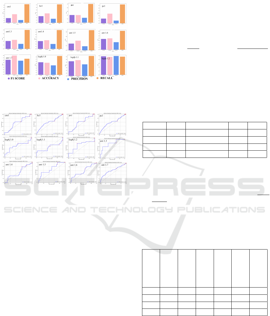
Figure 5: Evaluation metrics with supplementary Pareto ap-

proach and optimized parameter k. Purple: F1-score; Pink:

Accuracy; Blue: Precision; Orange: recall; the bars de-

scribe the scores on a scale from 0 to 1.0.

Figure 6: ROC AUC for COF with supplementary Pareto

approach and optimized parameter k: 0X-axis deﬁnes the

False Positive Rate, 0Y-axis denotes the True Positive Rate

more instances in the provided dataset, the higher the

required value for k.

The recall of 80% that was originally intended is

undoubtedly reached; however, the rest of the met-

rics are not as high, except for projects LOG4J and

ANT1.7. A second particularity of these datasets is

the high number of defects (in Table 1 Log4j clus-

ter has defects of 25% up to 92%, compared to

projects CM1, JM1, KC1, PC1 that have between 8

and 18,34% defects).

4.4 Comparison with Traditional

Methods

This section presents the results obtained along with

the latest results, namely the isolation forest (and the

improved isolation forest (Ding et al., 2019), BiGAN

(Zhang et al., 2022), One-Class SVM (Moussa et al.,

2022). Additionally, we will also provide a com-

parison with other classic approaches such as Gaus-

sian Naive Bayes, Logistic Regression, KNeighbours

Classiﬁer, and Decision Tree Classiﬁer according to

the results documented by Afric et al. (Afric et al.,

2020).

The projects used to compare the results are CM1,

KC1, JM1, and PC1, being an intersection of projects

from previously proposed approaches and the propos-

als in this study.

Table 2 contains the results of our approaches,

namely in column COF and in column COF+Pareto,

and the result of the Univariate Gaussian Distri-

bution(UGD) and Multivariate Gaussian Distribu-

tion(MGD) for the same task. It may be noticed that

our base approach outperforms both UGD and MGD

in terms of accuracy.

Table 2: Accuracy table that compares our base approach

to LOF, LOF enhanced by the Pareto rule, Univariate Gaus-

sian Distribution (with selected attributes), and Multivariate

Gaussian Distribution (with selected attributes) from (Neela

et al., 2017).

Dataset COF COF+Pareto UGD MGD

CM1 0.895 0.61 0.744 0.658

KC1 0.849 0.59 N/A N/A

JM1 0.808 0.60 0.780 0.740

PC1 0.925 0.785 0.756 0.600

Our overall f1-score is rather low for both of the

approaches, compared to most of the existing meth-

ods e.g., results for Bagging, Boosting, Random For-

est, and Isolation Forest (Ding et al., 2019). The com-

parison between our approaches, i.e. columns COF

and COF2 and the others in Table 3 reﬂects these re-

sults. The weakness of our proposed method is simi-

larly highlighted in Table 4a.

Table 3: F1-score values comparing our results with the

ones from (Ding et al., 2019), i.e. Bagging, Boosting, Ran-

dom Forest, Isolation forest with an ensemble scale of 150,

as it produced the maximum values.

Dataset

COF

COF + Pareto

Bagging

Boosting

CM1 0.29 0.33 0.65 0.67 0.68 0.71

KC1 0.38 0.26 0.75 0.74 0.75 0.75

JM1 0.40 0.45 0.70 0.65 0.67 0.72

PC1 0.31 0.42 0.62 0.60 0.65 0.69

Table 5 and Table 4b show the ROC AUC val-

ues, comparing our results with those of (Ding et al.,

2019), respectively, with those of (Zhang et al., 2022).

The results for datasets such as CM1 and KC1 may

be considered acceptable to good, compared to the

results of other studies. It is worth noting that the

values from these NASA datasets (CM1, KC1, JM‘,

PC1) are the lowest values for ROC AUC, contrary

Outlier Detection Through Connectivity-Based Outlier Factor for Software Defect Prediction

481

Table 4: Comparison of our results with the ones from (Zhang et al., 2022), i.e. RFB (RF + Balance), SVMB (SVM +

Balance), RFS (RF + SMOTE), SVMS (SVM + SMOTE), RFU (RF + Undersampling) and their proposed ADGAN.

Set COF COF2 RFB SVMB RFS SVMS RFU ADGAN

CM1 0.29 0.33 0.069 0.287 0.192 0.274 0.296 0.451

KC1 0.38 0.26 N/A N/A N/A N/A N/A N/A

JM1 0.40 0.45 0.257 0.351 0.378 0.347 0.401 0.408

PC1 0.31 0.42 0.181 0.291 0.398 0.302 0.312 0.238

(a) F1-score values

Set COF COF2 RFB SVMB RFS SVMS RFU ADGAN

CM1 0.66 0.57 0.507 0.628 0.536 0.611 0.636 0.700

KC1 0.66 0.59 N/A N/A N/A N/A N/A N/A

JM1 0.81 0.75 0.561 0.594 0.606 0.592 0.610 0.631

PC1 0.62 0.75 0.554 0.699 0.703 0.704 0.740 0.703

(b) AUC values

to the results retrieved by experimenting with Apache

project datasets such as Log4j or Ant.

Table 5: AUC values comparing our results with the ones

from (Ding et al., 2019), i.e. Bagging, Boosting, Random

Forest, Isolation forest with an ensemble scale of 150, as it

produced the maximum values.

Dataset

COF

COF+Pareto

Bagging

Boosting

CM1 0.66 0.57 0.72 0.69 0.81 0.87

KC1 0.66 0.59 0.84 0.79 0.83 0.89

JM1 0.81 0.75 0.74 0.85 0.84 0.90

PC1 0.62 0.75 0.87 0.81 0.83 0.88

We can conclude that the COF performs better on

small data, as we observe in Figure 4 and Figure 6,

showing that the fewer points, the higher the curve.

5 THREATS TO VALIDITY

Each experimental analysis can suffer from some va-

lidity threats and biases that can affect the study re-

sults. Several issues are provided that could affect

the results obtained and the actions taken to mitigate

them.

Internal validity may be at risk in our case due

to factors such as parameter settings or implementa-

tion issues. For the second approach, the experiments

from the original study were reproduced using the

same datasets and parameter settings, meaning that

the Pareto Principle only supports setting the thresh-

old, i.e. contamination or connectivity parameter to

20. Thus, our originality is in the implementation de-

sign and the application of the method with the addi-

tional parameter to the SDP problem.

External validity is related to the generalization of

the results obtained. The following key issues are

identiﬁed as possible threats to validity: the evalu-

ation measures used and the datasets. The selected

evaluation measures are the same as those in the pa-

pers used for the comparisons. As in these papers, the

same projects from the same repositories (NASA and

PROMISE) were used. However, other repositories

could also be considered in the future.

6 CONCLUSIONS

Software testing is a costly activity, especially

when continuous development or maintenance is per-

formed. Automated testing may cover regression test-

ing, but it is still an explicit step-by-step solution

that becomes more expensive when adapted to large

changes, such as code refactoring. To simplify these

processes, supervised or unsupervised binary classi-

ﬁcation software defect prediction (SDP) techniques

can rule out defective components or highlight the

least defective components. In this paper, outlier de-

tection methods for SDP were investigated. The nov-

elty of this approach is that it was not previously used

for this particular task. Two approaches were used:

simple use of the local outlier factor based on con-

nectivity (COF) and then enhancement by the Pareto

rule (which means that we consider samples with the

20% highest outlier score resulting from the algorithm

as outliers), COF + Pareto. Multiple projects from

the NASA and PROMISE datasets were used to val-

idate the proposed approaches. The results obtained

are comparable to state-of-the-art solutions.

ENASE 2024 - 19th International Conference on Evaluation of Novel Approaches to Software Engineering

482

ACKNOWLEDGMENT

This work was funded by the Ministry of Research,

Innovation, and Digitization, CNCS/CCCDI - UE-

FISCDI, project number PN-III-P1-1.1-TE2021-0892

within PNCDI III.

REFERENCES

Afric, P., Sikic, L., Kurdija, A. S., and Silic, M.

(2020). Repd: Source code defect prediction as

anomaly detection. Journal of Systems and Software,

168:110641.

Agrawal, A. and Menzies, T. (2018). Is” better data” better

than” better data miners”? on the beneﬁts of tuning

smote for defect prediction. In Proceedings of the

40th International Conference on Software engineer-

ing, pages 1050–1061.

Berrar, D. (2019). Cross-validation.

Breunig, M. M., Kriegel, H.-P., Ng, R. T., and Sander, J.

(2000). Lof: identifying density-based local outliers.

In Proceedings of the 2000 ACM SIGMOD interna-

tional conference on Management of data, pages 93–

104.

Dimitrov, M. and Zhou, H. (2009). Anomaly-based bug

prediction, isolation, and validation: an automated ap-

proach for software debugging. In Proceedings of the

14th international conference on Architectural sup-

port for programming languages and operating sys-

tems, pages 61–72.

Ding, Z. (2021). Isolation forest wrapper approach for fea-

ture selection in software defect prediction. In IOP

Conference Series: Materials Science and Engineer-

ing, volume 1043, page 032030. IOP Publishing.

Ding, Z., Mo, Y., and Pan, Z. (2019). A novel software

defect prediction method based on isolation forest.

In 2019 International Conference on Quality, Re-

liability, Risk, Maintenance, and Safety Engineering

(QR2MSE), pages 882–887. IEEE.

Ding, Z. and Xing, L. (2020). Improved software defect pre-

diction using pruned histogram-based isolation forest.

Reliability Engineering & System Safety, 204:107170.

Doshi-Velez, F. and Perlis, R. H. (2019). Evaluating ma-

chine learning articles. Jama, 322(18):1777–1779.

Gupta, N., He, H., Zhang, X., and Gupta, R. (2005). Locat-

ing faulty code using failure-inducing chops. In Pro-

ceedings of the 20th IEEE/ACM international Confer-

ence on Automated software engineering, pages 263–

272.

Han, S., Hu, X., Huang, H., Jiang, M., and Zhao, Y. (2022).

Adbench: Anomaly detection benchmark. Advances

in Neural Information Processing Systems, 35:32142–

32159.

Khan, M. E. and Khan, F. (2014). Importance of software

testing in software development life cycle. Interna-

tional Journal of Computer Science Issues (IJCSI),

11(2):120.

Kitchenham, B. A. and Charters, S. (2007). Guidelines for

performing systematic literature reviews in software

engineering. Technical Report EBSE 2007-001, Keele

University and Durham University Joint Report.

Kramer, O. and Kramer, O. (2016). Scikit-learn. Machine

learning for evolution strategies, pages 45–53.

Menzies, T., Greenwald, J., and Frank, A. (2006). Data

mining static code attributes to learn defect predictors.

IEEE transactions on software engineering, 33(1):2–

13.

Moldovan, A. (2023). Outlier detection through

connectivity-based outlier factor for software defect

prediction.

Moldovan, A. and Vescan, A. (accessed December 2023).

Outlier detection through connectivity-based outlier

factor for software defect prediction.

Moshtari, S., Santos, J. C., Mirakhorli, M., and Okutan,

A. (2020). Looking for software defects? ﬁrst ﬁnd

the nonconformists. In 2020 IEEE 20th Interna-

tional Working Conference on Source Code Analysis

and Manipulation (SCAM), pages 75–86. IEEE.

Moussa, R., Azar, D., and Sarro, F. (2022). Investigating the

use of one-class support vector machine for software

defect prediction. arXiv preprint arXiv:2202.12074.

Myers, G. J., Sandler, C., and Badgett, T. (2011). The art

of software testing. John Wiley & Sons.

Neela, K. N., Ali, S. A., Ami, A. S., and Gias, A. U. (2017).

Modeling software defects as anomalies: A case study

on promise repository. J. Softw., 12(10):759–772.

Tang, J., Chen, Z., Fu, A. W.-C., and Cheung, D. W. (2002).

Enhancing effectiveness of outlier detections for low

density patterns. In Advances in Knowledge Discov-

ery and Data Mining: 6th Paciﬁc-Asia Conference,

PAKDD 2002 Taipei, Taiwan, May 6–8, 2002 Pro-

ceedings 6, pages 535–548. Springer.

Wahono, R. S. (2015). A systematic literature review of

software defect prediction. Journal of software engi-

neering, 1(1):1–16.

Wang, S., Liu, T., and Tan, L. (2016). Automatically learn-

ing semantic features for defect prediction. In Pro-

ceedings of the 38th International Conference on Soft-

ware Engineering, pages 297–308.

Zhang, S., Jiang, S., and Yan, Y. (2022). A software defect

prediction approach based on bigan anomaly detec-

tion. Scientiﬁc Programming, 2022.

Outlier Detection Through Connectivity-Based Outlier Factor for Software Defect Prediction

483