Real-Time Traffic Prediction Through Stochastic Gradient Descent
Yasmine Amor
1,4 a
, Lilia Rejeb
1 b
, Nabil Sahli
2 c
, Wassim Trojet
3 d
, Lamjed Ben Said
1 e
and
Ghaleb Hoblos
4 f
1
Universit
´
e de Tunis, Institut Sup
´
erieur de Gestion de Tunis, SMART Lab, Tunis, Tunisia
2
German University of Technology in Oman, Oman
3
Higher Colleges of Technology, U.A.E.
4
IRSEEM, Technopole du Madrillet, Av. Galilee, Saint-Etienne du Rouvray, Normandy, France
Keywords:
Online Learning Methods, Real-Time Data, Traffic Prediction, Stochastic Gradient Descent.
Abstract:
The escalating challenges of urban traffic congestion pose a critical issue that calls for efficient traffic man-
agement system solutions. Traffic forecasting stands out as a paramount area of exploration in the field of
Intelligent Transportation Systems. Various traditional machine learning techniques have been employed for
predicting traffic congestion, often requiring a significant amount of data to train the model. For that reason,
historical data are usually used. In this paper, our first concern is to use real-time traffic data. We adopted
Stochastic Gradient Descent, an online learning method characterized by its ability to continually adapt to
incoming data, facilitating real-time updates and rapid predictions. We studied a network of streets in the city
of Muscat, Oman. Our model showed its accuracy through comparisons with actual traffic data.
1 INTRODUCTION
In urban regions, traffic congestion has become a seri-
ous issue impacting economic activity, environmental
sustainability and quality of life. As cities burgeon
in size and complexity, the challenge of managing
and alleviating traffic congestion becomes an increas-
ingly difficult task. According to GITNUX data re-
port of 2024 (Castillo, 2024), traffic congestion costs
the average American commuter $1,377 per year in
wasted time and fuel. An overall value of 8 billion
hours is annually wasted by Americans due to traffic
congestion. The statistics are equally challenging for
the United Kingdom, where congestion is projected to
cost each driver £1,317 in 2030, resulting in a yearly
total of £4.4 billion. Additionally, Nairobi, Kenya,
faces an estimated annual cost of $1 billion due to
traffic congestion. Meanwhile, in Toronto, Canada,
traffic congestion costs the country a significant $6
a
https://orcid.org/0000-0002-0795-550X
b
https://orcid.org/0000-0002-5740-1556
c
https://orcid.org/0000-0002-9805-6859
d
https://orcid.org/0000-0001-7792-4402
e
https://orcid.org/0000-0001-9225-884X
f
https://orcid.org/0000-0003-3268-5270
billion annually.
Accordingly, the issue of traffic congestion has
led to increased interest and research in Intelligent
Transportation Systems (ITS), particularly in traffic
congestion forecasting. Real-time data plays a vital
role in effective traffic management, enabling quick
interventions to enhance traffic flow and alleviate con-
gestion. Therefore, predicting traffic congestion oc-
currence is crucial for addressing it effectively (Al-
berto, 2003). Various traditional methods have been
employed to forecast traffic patterns. However, the
problem is that the majority of them are trained on
a fixed data set and update their parameters based
on the entire data set at once, in contrast to, online
learning methods that continuously adapt to incom-
ing data in a sequential manner, allowing real-time
updates and quick predictions. Online learning meth-
ods are, therefore, commonly used when dealing with
real time data. These methods were used in various
domains such as virtual energy storage capacity, med-
ical data analysis, flight control, etc. In this paper,
our objective is to explore the application of online
learning methods in predicting roads traffic conges-
tion. We use real time data from the Google Maps
API. Traffic congestion prediction is handled in our
paper by the implementation of Stochastic Gradient
Amor, Y., Rejeb, L., Sahli, N., Trojet, W., Ben Said, L. and Hoblos, G.
Real-Time Traffic Prediction Through Stochastic Gradient Descent.
DOI: 10.5220/0012687400003702
Paper published under CC license (CC BY-NC-ND 4.0)
In Proceedings of the 10th International Conference on Vehicle Technology and Intelligent Transport Systems (VEHITS 2024), pages 361-369
ISBN: 978-989-758-703-0; ISSN: 2184-495X
Proceedings Copyright © 2024 by SCITEPRESS – Science and Technology Publications, Lda.
361

Descent (SGD) algorithm. The obtained output re-
sults are compared with real traffic values, showing
accurate and effective prediction results.
The paper is organized as follows: Section 2
presents a literature review of the existing methods.
Section 3 describes some of the online learning meth-
ods used for prediction in different domains, high-
lighting the advantages of applying these methods in
the domain of traffic congestion prediction. Section
4 presents the case study, describing the studied net-
work, the principle of features generation and pre-
diction horizons calculation, and the use of SGD for
traffic prediction. In section 5, we show the results
generated by our model. Finally, Section 6 presents
the conclusions derived from this study and some per-
spectives.
2 STATE OF THE ART
Traffic congestion forecasting has led to a grow-
ing research area. Various machine learning models
have been used to predict traffic. Some of the most
used methods include Time Series Analysis methods,
specifically AutoRegressive Integrated Moving Av-
erage (ARIMA) and Seasonal ARIMA (SARIMA),
which are valued for their simplicity and interpretabil-
ity. Alghamdi et al. (Alghamdi et al., 2019) treated
the problem of traffic congestion using ARIMA-based
modeling for non-Gaussian traffic data. They focused
on short-term predictions, exploring factors that in-
fluenced congestion. The authors based their model
on Auto Correlation Function (ACF) and Partial Auto
Correlation Function (PACF) analyses of hourly traf-
fic flow observations in a specific roads network of
California, USA. Zhou et al. (Zhou et al., 2005)
developed a traffic prediction model, combining lin-
ear time series ARIMA with the non-linear Gener-
alized Auto Regressive Conditional Heteroscedastic-
ity (GARCH). This hybrid model was able to cap-
ture various traffic characteristics at both large and
small scales, addressing the complexity of network
behavior. ARIMA models were suitable for model-
ing temporal patterns due to their simplicity and in-
terpretability. They were particularly efficient for cap-
turing regularities in historical traffic data. However,
their shortcomings become apparent when we deal
with complex non-linear relationships present in dy-
namic and rapidly changing road traffic conditions.
In situations where traffic patterns are dynamic, these
methods might find it difficult to adjust to the varia-
tion of real-time traffic data.
Other approaches for predicting traffic congestion
include the utilization of Neural Networks. Various
architectures of neural networks were proposed in
the literature, such as Feedforward Neural Networks
(FNN) (Louati et al., 2022) (Olayode et al., 2022),
Recurrent Neural Networks (RNN) (Lu et al., 2021)
(Guo et al., 2020), and Long Short-Term Memory
(LSTM) networks (Sunindyo and Satria, 2020) (Afrin
and Yodo, 2022).
Oliveira et al. (Oliveira et al., 2016) conducted
a comparative study between the existing types of
neural networks used for forecasting network traf-
fic. The studied models included Multi Layer Percep-
tron (MLP) with backpropagation, MLP with resilient
backpropagation (Rprop), Recurrent Neural Network
(RNN), and deep learning Stacked Auto Encoder
(SAE). (Redhu et al., 2023) proposed a model en-
titled Multi-View Dynamic Graph Convolution Net-
work (MVDGCN). It addresses the complex spatial-
temporal patterns in traffic flow. The authors used
Graph Convolution Network (GCN) to understand the
relationships between the different traffic stations in
the studied network, which helped them to capture
spatial dependencies. The authors used historical
datasets (NYCTaxi and NYCBike). GCNs showed
accurate results. However, the computational com-
plexity of these models makes them less suitable for
real-time applications. Fan et al. (Fan et al., 2019) de-
veloped a prediction model leveraging a combination
of deep RNN and Gated Recurrent Unit (GRU) neural
network techniques. The proposed model aims to de-
tect network failures, optimize the performance, and
enhance the overall network security through accurate
traffic prediction. The model was validated by com-
paring prediction values with actual traffic values in
real-world environments. This approach showcased
the potential of neural network-based models. How-
ever, challenges for such models may include compu-
tational intensity, especially in real-time applications,
and the complex training process associated with deep
neural networks.
Other prediction models used Random Forests
(Evans et al., 2019) (Hamad et al., 2020) and Support
Vector Machines (Zhu and Zheng, 2020) (Radzuan
et al., 2020) to predict traffic.
Evans et al. (Evans et al., 2019) focused on eval-
uating the RoadCast algorithm, which is an existing
random forest algorithm. RoadCast was specifically
developed to forecast road traffic conditions several
hours, days, or even months in advance. The bene-
fit of this work was that RoadCast’s forecasting accu-
racy was improved by incorporating contextual data,
such as public holidays and events, which increases
its ability to adjust to variations in real-world traf-
fic conditions. In contrast, the effectiveness of this
algorithm was highly dependent on the quality and
VEHITS 2024 - 10th International Conference on Vehicle Technology and Intelligent Transport Systems
362

availability of data. Variability in data quality and
quantity could impact the algorithm’s performance.
Chen et al. (Chen et al., 2019) analyzed the spatio-
temporal correlation properties of traffic states us-
ing floating cars data. The paper introduced an en-
hancement of the random forest algorithm, address-
ing the spatio-temporal correlation features of urban
road traffic states.
To summarize, despite their high predictive accu-
racy, Random Forests (RFs) pose some challenges for
traffic congestion prediction. Training a Random For-
est with a large number of trees and features may
be computationally expensive. In real-time applica-
tions, where quick predictions are crucial, the compu-
tational complexity of the model may be a limitation.
In addition, the performance of Random Forest mod-
els is highly dependent on the quality, and quantity of
the training data. If the training data are insufficient to
fully represent the variability of traffic conditions, the
model’s predictive performance may be sub-optimal.
Apart from the previously mentioned models,
there are other methods for traffic prediction, such
as Bayesian Networks (Kim and Wang, 2016) (Afrin
and Yodo, 2021), Genetic Algorithms (Lopez-Garcia
et al., 2015) (Abdulhai et al., 2002) and K-Nearest
Neighbors (Priambodo and Jumaryadi, 2018) (Yu
et al., 2016), etc.
All the presented models were able to capture
complex patterns and relationships in underlying traf-
fic data. They are effective for both short-term and
long-term traffic predictions. However, they require
a large amount of data for training, which explains
the use of historical data for almost all of them. Nev-
ertheless, these methods might struggle to capture the
dynamic nature of traffic states when dealing with real
time data. Using real-time data increases complexity
and, thus, requires careful consideration of the rapid
changes of road conditions. For this matter, we are
considering the use of online learning methods that
are known for their ability to handle real time data.
In the next section, we introduce some studies
that employed online learning methods for prediction
across diverse domains. Subsequently, we delve into
the specific method used in our study.
3 ONLINE LEARNING METHODS
Online Learning represents a dynamic paradigm
within machine learning, where models are updated
continuously as new data becomes available, enabling
real-time updates and short-time predictions. In on-
line learning, the model receives data in a sequential
manner, one sample at a time, and updates its parame-
ters based on each new sample. This stands in contrast
to traditional learning models, where the model trains
on a fixed data set and updates its parameters using the
entire data set simultaneously. Online learning is par-
ticularly valuable for scenarios where data fluctuates
over time and where rapid predictions are needed.
There are several online learning methods that
have been used for prediction tasks, such as SGD,
Adaptive Gradient Descent (ADAGRAD), Online
Passive-Aggressive (PA), RMSprop (Root Mean
Square Propagation), AdaDelta, etc. Some of these
models were used in the literature to generate pre-
dictions in different domains, such as the prediction
of virtual energy storage capacity, health data anal-
ysis, Predicting kids malnutrition, flight control, etc.
Khan et al. (Khan et al., 2022) focused on the analysis
of medical data. They proposed a machine learning-
based stochastic gradient descent method in order
to manage medical records and optimize day-to-day
transactions in e-Healthcare applications. Vijayalak-
shmi et al. (Vijayalakshmi et al., 2022) addressed
the challenges associated with the integration of re-
newable energy sources (RES) in smart grids. They
developed a model that uses Artificial Neural Net-
work (ANN) and SGD to predict Air Conditioners
energy capacity, facilitating the Virtual Energy Stor-
age System VESS implementation. Fawazdhia et al.
(Fawazdhia and HSM, 2023) studied the prediction of
stock prices. They employed both SGD and Adam
optimization. The final results showed that values
of the next day’s stock prices were successfully pre-
dicted.
In summary, online learning methods have been
successful in providing real-time adaptability to
changing data, allowing continuous model updates
and rapid responses to evolving patterns. Taking ad-
vantage of this, our aim in this work is to employ
these methods in the transportation field. In partic-
ular, we use SGD to predict traffic congestion in the
city of Muscat, Oman. The dynamic nature of SGD
aligns well with the real-time aspects of traffic pat-
terns. As new traffic data becomes available, SGD
allows more accurate predictions and enhances the
system’s responsiveness to sudden changes in traffic
conditions.
In the next section, we present the used data, the
principle of traffic congestion estimation and predic-
tion, and the results obtained by using our system.
Real-Time Traffic Prediction Through Stochastic Gradient Descent
363

4 TRAFFIC PREDICTION IN
MUSCAT, OMAN
We conducted our study on a network of roads in
Muscat, Oman. Figure 1 illustrates the general archi-
tecture of our network system. We are using Smart
Road Signs (SRSs) which serve as the main compo-
nent in the studied roads network (Hamdani et al.,
2022).
Figure 1: The studied Roads Network, Muscat, Oman.
These Smart Road Signs are able to collect real-
time traffic data, estimate traffic conditions and pre-
dict congestion across various time horizons based on
the current traffic status. When compared to the cur-
rent Dynamic Message Signs (DMSs), that display
the traffic condition as determined by traffic manage-
ment centers, the Smart Road Signs we are using pos-
sess intelligence and autonomy, which enables them
to analyze data and forecast future traffic values.
The studied road traffic network comprises seven
roundabouts, considered as significant contributors to
traffic congestion. We placed one Smart Road Sign
before each roundabout so that it can alert drivers
heading towards that roundabout. Each Road Sign
receives information about the traffic conditions in
its own studied road and the roads occupied by its
neighboring road signs. In order to enhance predic-
tion accuracy, Smart Road Signs communicate with
each others and collaborate to give effective results.
The studied direction of traffic is represented by black
arrows in the same figure.
The developed Smart Road Signs are currently in
a simulation phase. The solution is not deployed in a
real operational environment. We are testing and eval-
uating their performance under real conditions. This
phase allows for the assessment of the system’s func-
tionality, performance, and predictive capabilities be-
fore potential real-world deployment.
In the following, we present the used data, the fea-
tures generation process, the principle of prediction
horizons identification and the use of SGD for traffic
prediction.
4.1 Used Data
In order to get real time traffic data, we used Google
Maps API. We considered the Directions API and API
distance matrix
1
. These APIs provide the Travel Dis-
tance and Travel Time for a matrix of origins and des-
tinations. Using Google Map API, we obtain informa-
tion on the studied roads between the specified start
and end points (the roundabouts).
4.2 Features Generation and Prediction
Horizons Calculation
In this section, we present the principle of features
calculation, their exploitation per road signs and the
prediction horizons definition.
4.2.1 Features Calculation
Google Maps API offers Travel Time between two
points, providing two types: estimated Travel Time,
reflecting standard travel duration under free-flow
road conditions, and actual real Travel Time, showing
the real-time duration vehicles take to travel between
points.
Knowing the actual real Travel Time value, we can
calculate the average speed and compare it with the
maximum allowed speed in the same road. This is
how our features are generated.
Equation 1 illustrates the calculation of our features.
F
i, j
=
"

T D
i, j
T T
i, j

1
V
max
i, j
#
× 100, (1)
where:
F
i, j
is the feature from point i to point j.
T D
i, j
is the Travel Distance between the two points i
and j.
T T
i, j
is the actual real Travel Time from point i to
point j.
V
max
i, j
is the maximum permissible speed in the road
from point i to point j.
The final value of the feature is between 0 and 100,
but may exceed 100 if the vehicle drivers are surpass-
ing the maximum allowed speed in the studied road.
According to (He et al., 2016), such value can be clas-
sified according to three threshold values: 25, 50, and
75. If the feature is between 0 and 25, it indicates a
heavy congestion. If it is between 25 and 50, the traf-
fic presents a mild congestion. Otherwise, we have a
smooth to very smooth traffic condition.
All the seven road signs of our network work si-
multaneously. Each road sign generates three distinct
1
https://developers.google.com/maps
VEHITS 2024 - 10th International Conference on Vehicle Technology and Intelligent Transport Systems
364

features taken at different timestamps. Based on the
time windows between these times, we determine our
prediction horizons. We describe this principle in de-
tail in the next subsection.
4.2.2 Prediction Horizons Calculation
Let f
i
represent the feature generated at time t
i
by a
given road sign, where i varies from 1 to n, and n is
the number of features. The time window for gen-
erating the next feature is determined by checking in
which range the current feature falls. Thus, the time
window for generating the next feature, f
i+1
, is deter-
mined based on the value of f
i
:
t
i+1
= t
i
+





1 minute if 0 ≤ f
i
< 25,
5 minutes if 25 ≤ f
i
< 50,
10 minutes if f
i
≥ 50.
(2)
The process continues by generating subsequent
features based on the previous ones. Predictions are
made after every set of three features generated by
each road sign at the different timestamps. The pre-
diction horizon for each set, PH
k
, is calculated by
summing the time windows of the three different fea-
tures:
PH
k
=
3
∑
i=1
∆t
k,i
, (3)
where k represents the index of the feature set and ∆t
k,i
is determined by the value of the feature according to
the specified traffic conditions.
In the next section, we explain the use of SGD to
predict Traffic congestion.
4.3 Real-Time Traffic Prediction Using
SGD
We studied traffic in the roads presented in Figure 1,
mainly Al Khoudh Street, Al Mazoon Sreet, and al
Shabab Street. The studied scenario covers the time
period from 08/11/2023 09:00 to 08/11/2023 11:00.
Road signs gather real time data from Google
Maps API, calculate features and predict traffic each
set of three features.
The generation of the prediction values for one set
of three features is given by Algorithm 1. It shows
the most important steps for the traffic prediction with
SGD.
The Inputs of our system consists of the real-time
data recorded from 09:00 AM to 11:00 AM since this
period of the day is considered as peak hour. In turn,
the system generates as output prediction values of
the seven deployed road signs.
The first step is the initialization of our sys-
tem. We import necessary libraries: torch,
torch.nn.functional, torch geometric.data, pandas,
and numpy. Afterward, we define the number of fea-
tures and the number of output predictions. In this
case, as we consider a set of three features for each
road sign, the number of features per road sign is 3,
and the number of output predictions is 1. This pro-
cess is then iterated over time to make all necessary
predictions within the studied period.
The next step involves generating features for each
road sign, where feature arrays are transformed into
PyTorch tensors. Following this, a data instance ob-
ject is created, encompassing the data from all work-
ing road signs within our network.
In the definition of the OnlineSGD model,
we start by establishing the OnlineSGD
class, equipped with fit and predict methods.
Data: Real Time Data from External Source
Result: Traffic Prediction Values
Initialization;
Define number of features (num features);
Define number of output predictions
(num
Predictions);
Generate features for each node:
X ← generate features();
Create a Data instance object from features:
data ← Data(x = X);
Initialize the OnlineSGD model:
model ← OnlineSGD(learning rate =
0.01, num epochs = 1000);
Train the model:
model.fit(data.x);
Test the model:
predictions ← model.predict(data.x);
for i in range(len(predictions)) do
Print prediction:
print(predictions[i]);
end
Algorithm 1: OnlineSGD for Traffic Congestion Prediction.
Our system’s performance depends on two key pa-
rameters: the learning rate and the number of epochs,
set during model initialization. After testing various
values, we fixed the learning rate (α) at 0.01 and
the number of epochs at 1000. During fitting, the
model iterates through epochs and instances, updat-
ing weights using stochastic gradient descent (SGD)
and calculating loss every 100 epochs. In the predic-
tion method, predictions are made using the learned
weights.
Real-Time Traffic Prediction Through Stochastic Gradient Descent
365

5 RESULTS AND DISCUSSION
In this section, we showcase the outcomes of our
model. Figures 2 to 8 show the results of prediction
generated by the seven road signs placed in our net-
work. Curves in blue represent the prediction values
generated by our model. The ones in red represent the
real values of roads’ traffic.
Figure 2: Traffic prediction values and real traffic values of
Road Sign 1.
Figure 3: Traffic prediction values and real traffic values of
Road Sign 2.
Figure 4: Traffic prediction values and real traffic values of
Road Sign 3.
Figure 5: Traffic prediction values and real traffic values of
Road Sign 4.
Figure 6: Traffic prediction values and real traffic values of
Road Sign 5.
Figure 7: Traffic prediction values and real traffic values of
Road Sign 6.
Figure 8: Traffic prediction values and real traffic values of
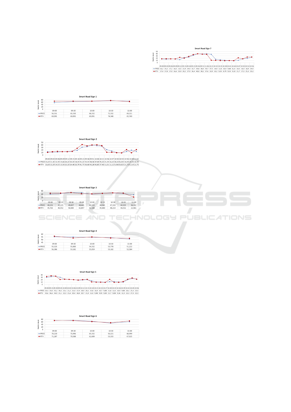
Road Sign 7.
If we take a look at the predicted traffic values of
Road Sign 1 (Figure 2) at different times, we can see
that the prediction at 09:00 shows a small gap from
the actual value, when compared to the other points
in the graph. Subsequent predictions get closer to
reality by the time and we can clearly see that the
points of prediction and real values almost overlap.
Notably, the 10:00 and 10:30 predictions are very ac-
curate, aligning closely with the real traffic. Other
road signs showed closer results, Road Sign 4 and 6
show five predictions during the studied period. Pre-
dicted values by Road Sign 4 are very close to the real
traffic values. For the Road Sign 6, they are almost
overlapped.
Examining Figure 2, a noteworthy observation is
the significant difference in the number of predictions
between Road Sign 1 and other road signs, like Road
Sign 4 and Road Sign 6. Road Sign 2 generates 19
prediction values within a 2-hour period. The short
prediction horizons for this road signs indicate severe
congestion on the studied road. Initial traffic values
range from 10.636 to 14.489, escalating to 41.739,
which is considered as a mild congestion, before re-
turning to lower traffic values.
The curves in Figure 3 illustrate how the predic-
tions mirror the traffic fluctuations. However, a no-
table deviation occurs at 10:59, where our model pre-
dicts a value of 19.332, while the actual traffic value is
9.114. This is explained by the sudden traffic change
from 21.736 to 9.114 within a short time.
Figure 4 illustrates the outcomes associated with
Road Sign 3. Deviations between prediction and real
traffic values are clear for the last instance (at 11:00).
The real traffic has the value of 22.981 whereas our
prediction value is 36.332. Examining the preceding
traffic value reveals a sharp decline from 46.552 to
22.981, indicating a sudden decrease. Although our
model detects this decrease in traffic, the predicted
value remains somewhat distant from the real traffic
value.
Similar scenarios were observed at 10:30 for Road
Sign 5 (Figure 6) and at 09:12 and 10:47 for Road
Sign 7 (Figure 8). In all these instances, the issue is
associated with an unexpected deviation in the values
of real traffic.
Overall, our model demonstrated accurate results
VEHITS 2024 - 10th International Conference on Vehicle Technology and Intelligent Transport Systems
366

in predicting traffic, with prediction values consis-
tently following the curve of the real traffic data.
However, a challenge arises in cases where the traf-
fic behaves unexpectedly, exhibiting sudden increases
or decreases. In such instances, the model doesn’t
always detect these abrupt changes. Future work
could address this limitation by incorporating addi-
tional data, such as weather conditions or incident re-
ports. Alternatively, combining the SGD with other
methods might be interesting and could enhance the
model’s ability to capture and respond to such abrupt
variations.
In order to give a more comprehensive under-
standing of the model’s accuracy, we used the Mean
Absolute Error (MAE) metric.
The Mean Absolute Error is calculated by taking
the absolute difference between the predicted values
and the actual values and then averaging those dif-
ferences. In other words, MAE quantifies the aver-
age magnitude of errors made by a predictive model.
When the MAE value is low, it indicates that, on av-
erage, the model’s predictions are close to the actual
values. This suggests a higher level of accuracy in the
model’s ability to estimate outcomes. On the contrary,
a higher MAE implies that the model tends to make
predictions that are, on average, farther away from the
actual values.
The MAE is given by equation 4.
MAE =
1
n
n
∑
i=1
|y
i
− ˆy
i
|, (4)
where:
• n is the number of total predictions.
• y
i
represents the real value of traffic.
• ˆy
i
represents the predicted value of traffic.
Table 1 presents the Mean Absolute Error (MAE)
values corresponding to each operational road sign
within the studied network. The analysis of these
values reveals insights into the predictive accuracy of
each sign.
Table 1: Mean Absolute Error Values of the generated Road
Signs.
SRS1 SRS2 SRS3 SRS4 SRS5 SRS6 SRS7
MAE 4.57 4.24 3.75 1.11 2.58 3.05 3.97
Notably, SRS4 stands out with the lowest MAE
of 1.11, indicating highly accurate predictions. This
suggests that the road sign 4 performs very well in es-
timating traffic conditions.
In comparison, SRS1 and SRS2, have higher MAE
values, respectively 4.57 and 4.24, suggesting less
precision in forecasting compared to SRS4. However,
it is important to note that, given the nature of the traf-
fic values ranging from 0 to 100, these MAE values
for SRS1 and SRS2 still fall within a good range. The
analysis further reveals that SRS3, SRS5, SRS6, and
SRS7 lie in between the aforementioned extremes.
To sum up, our smart road signs showcase a range
of performances, with some yielding more accurate
predictions than others.
Understanding MAE values for each road sign is
crucial for evaluating our predictive model’s reliabil-
ity in estimating traffic conditions. Our model has
shown impressive effectiveness in this context.
6 CONCLUSIONS
This paper suggested the use of online learning tech-
niques in the field of transportation. We developed
a model based on Stochastic Gradient Descent to pre-
dict the traffic congestion. We used Smart Road Signs
that collaborate to cover a road network in the city of
Muscat, Oman. Real time data were gathered from
Google Maps API. They were exploited to generate
features that served for the prediction phase. We
emphasize the use of real time data since it enables
timely insights and dynamic route adjustments. It can
also facilitate data-driven decision-making, benefiting
from up-to-the-minute information, which contributes
to effective urban mobility management. Seven road
signs were placed in our Network. Each of them gen-
erated a number of prediction considering different
prediction horizons. The reached results were com-
pared with real traffic values. Our system showed
its accuracy in predicting traffic congestion. By hav-
ing a data that changes frequently, our model showed
its performance to adapt to the new incoming data.
As future work, we aim to use other online learn-
ing methods such as ADaptive GRAdient Descent.
We also intend to work on different context and road
types.
ACKNOWLEDGEMENTS
The research leading to these results has received
funding from the Ministry of Higher Education,
Research and Innovation (MoHERI) of the Sul-
tanate of Oman under the Block Funding Pro-
gram. MoHERI Block Funding Agreement No
[BFP/RGP/ICT/22/327].
Real-Time Traffic Prediction Through Stochastic Gradient Descent
367

REFERENCES
Abdulhai, B., Porwal, H., and Recker, W. (2002). Short-
term traffic flow prediction using neuro-genetic algo-
rithms. ITS Journal-Intelligent Transportation Sys-
tems Journal, 7(1):3–41.
Afrin, T. and Yodo, N. (2021). A probabilistic estimation of
traffic congestion using bayesian network. Measure-
ment, 174:109051.
Afrin, T. and Yodo, N. (2022). A long short-term memory-
based correlated traffic data prediction framework.
Knowledge-Based Systems, 237:107755.
Alberto, B. (2003). Traffic congestion. In THE PROBLEM
AND HOW TO DEAL WITH IT, page 198.
Alghamdi, T., Elgazzar, K., Bayoumi, M., Sharaf, T., and
Shah, S. (2019). Forecasting traffic congestion us-
ing arima modeling. In 2019 15th international wire-
less communications & mobile computing conference
(IWCMC), pages 1227–1232. IEEE.
Castillo, L. (2024). Must-know traffic congestion statistics.
Retrieved from https://gitnux.org/traffic-congestion-s
tatistics/.
Chen, Z., Jiang, Y., and Sun, D. (2019). Discrimination and
prediction of traffic congestion states of urban road
network based on spatio-temporal correlation. IEEE
Access, 8:3330–3342.
Evans, J., Waterson, B., and Hamilton, A. (2019). Forecast-
ing road traffic conditions using a context-based ran-
dom forest algorithm. Transportation planning and
technology, 42(6):554–572.
Fan, J., Mu, D., and Liu, Y. (2019). Research on network
traffic prediction model based on neural network. In
2019 2nd International Conference on Information
Systems and Computer Aided Education (ICISCAE),
pages 554–557. IEEE.
Fawazdhia, M. A. A. and HSM, Z. A. R. (2023). Long short
term memory using stochastic gradient descent and
adam for stock prediction. CAUCHY: Jurnal Matem-
atika Murni dan Aplikasi, 8(2):16–29.
Guo, K., Hu, Y., Qian, Z., Liu, H., Zhang, K., Sun, Y.,
Gao, J., and Yin, B. (2020). Optimized graph convo-
lution recurrent neural network for traffic prediction.
IEEE Transactions on Intelligent Transportation Sys-
tems, 22(2):1138–1149.
Hamad, K., Al-Ruzouq, R., Zeiada, W., Abu Dabous, S.,
and Khalil, M. A. (2020). Predicting incident duration
using random forests. Transportmetrica A: transport
science, 16(3):1269–1293.
Hamdani, M., Sahli, N., Jabeur, N., and Khezami, N.
(2022). Agent-based approach for connected vehicles
and smart road signs collaboration. Computing and
Informatics, 41(1):376–396.
He, F., Yan, X., Liu, Y., and Ma, L. (2016). A traffic con-
gestion assessment method for urban road networks
based on speed performance index. Procedia engi-
neering, 137:425–433.
Khan, A. A., Laghari, A. A., Shafiq, M., Cheikhrouhou,
O., Alhakami, W., Hamam, H., and Shaikh, Z. A.
(2022). Healthcare ledger management: A blockchain
and machine learning-enabled novel and secure archi-
tecture for medical industry. Hum. Cent. Comput. Inf.
Sci, 12:55.
Kim, J. and Wang, G. (2016). Diagnosis and prediction
of traffic congestion on urban road networks using
bayesian networks. Transportation Research Record,
2595(1):108–118.
Lopez-Garcia, P., Onieva, E., Osaba, E., Masegosa, A. D.,
and Perallos, A. (2015). A hybrid method for short-
term traffic congestion forecasting using genetic algo-
rithms and cross entropy. IEEE Transactions on Intel-
ligent Transportation Systems, 17(2):557–569.
Louati, A., Masmoudi, F., and Lahyani, R. (2022). Traffic
disturbance mining and feedforward neural network
to enhance the immune network control performance.
In Proceedings of Seventh International Congress on
Information and Communication Technology: ICICT
2022, London, Volume 1, pages 99–106. Springer.
Lu, S., Zhang, Q., Chen, G., and Seng, D. (2021). A
combined method for short-term traffic flow predic-
tion based on recurrent neural network. Alexandria
Engineering Journal, 60(1):87–94.
Olayode, I. O., Severino, A., Campisi, T., and Tartibu,
L. K. (2022). Prediction of vehicular traffic flow using
levenberg-marquardt artificial neural network model:
Italy road transportation system. Komunik
´
acie, 24(2).
Oliveira, T. P., Barbar, J. S., and Soares, A. S. (2016).
Computer network traffic prediction: a comparison
between traditional and deep learning neural net-
works. International Journal of Big Data Intelligence,
3(1):28–37.
Priambodo, B. and Jumaryadi, Y. (2018). Time series traffic
speed prediction using k-nearest neighbour based on
similar traffic data. In MATEC Web of Conferences,
volume 218, page 03021. EDP Sciences.
Radzuan, N., Hassan, M., Musa, R., Majeed, A. A., Raz-
man, M. M., and Kassim, K. A. (2020). A support vec-
tor machine approach in predicting road traffic mortal-
ity in malaysia. Journal of the Society of Automotive
Engineers Malaysia, 4(2):135–144.
Redhu, P., Kumar, K., et al. (2023). Short-term traffic flow
prediction based on optimized deep learning neural
network: Pso-bi-lstm. Physica A: Statistical Mechan-
ics and its Applications, 625:129001.
Sunindyo, W. D. and Satria, A. S. M. (2020). Traffic
congestion prediction using multi-layer perceptrons
and long short-term memory. In 2020 10th Elec-
trical Power, Electronics, Communications, Controls
and Informatics Seminar (EECCIS), pages 209–212.
IEEE.
Vijayalakshmi, K., Vijayakumar, K., and Nandhakumar, K.
(2022). Prediction of virtual energy storage capacity
of the air-conditioner using a stochastic gradient de-
scent based artificial neural network. Electric Power
Systems Research, 208:107879.
Yu, B., Song, X., Guan, F., Yang, Z., and Yao, B. (2016). k-
nearest neighbor model for multiple-time-step predic-
tion of short-term traffic condition. Journal of Trans-
portation Engineering, 142(6):04016018.
VEHITS 2024 - 10th International Conference on Vehicle Technology and Intelligent Transport Systems
368

Zhou, B., He, D., Sun, Z., and Ng, W. H. (2005). Network
traffic modeling and prediction with arima/garch. In
Proc. of HET-NETs Conference, pages 1–10.
Zhu, Y. and Zheng, Y. (2020). Retracted article: traffic iden-
tification and traffic analysis based on support vec-
tor machine. Neural Computing and Applications,
32(7):1903–1911.
Real-Time Traffic Prediction Through Stochastic Gradient Descent
369