UoCAD: An Unsupervised Online Contextual Anomaly Detection

Approach for Multivariate Time Series from Smart Homes

Aafan Ahmad Toor

, Jia-Chun Lin

, Ming-Chang Lee

and Ernst Gunnar Gran

Department of Information Security and Communication Technology,

Norwegian University of Science and Technology, Gjøvik, Norway

Keywords:

Internet of Things, Smart Home, Long Short-Term Memory (LSTM), Online Learning, Time Series, Anomaly

Detection, Sliding Window.

Abstract:

In the context of time series data, a contextual anomaly is considered an event or action that causes a deviation

in the data values from the norm. This deviation may appear normal if we do not consider the timestamp

associated with it. Detecting contextual anomalies in real-world time series data poses a challenge because it

often requires domain knowledge and an understanding of the surrounding context. In this paper, we propose

UoCAD, an online contextual anomaly detection approach for multivariate time series data. UoCAD employs

a sliding window method to (re)train a Bi-LSTM model in an online manner. UoCAD uses the model to

predict the upcoming value for each variable/feature and calculates the model’s prediction error value for each

feature. To adapt to minor pattern changes, UoCAD employs a double-check approach without immediately

triggering an anomaly notiﬁcation. Two criteria, individual and majority, are explored for anomaly detection.

The individual criterion identiﬁes an anomaly if any feature is detected as anomalous, while the majority

criterion triggers an anomaly when more than half of the features are identiﬁed as anomalous. We evaluate

UoCAD using an air quality dataset containing a contextual anomaly. The results show UoCAD’s effectiveness

in detecting the contextual anomaly across different sliding window sizes but with varying false positives and

detection time consumption.

1 INTRODUCTION

A time series refers to a sequence of data points col-

lected and indexed in time order (Belay et al., 2023).

The Internet of Things (IoT) has become a major

source of time series data in recent times, as it has

been used in smart homes, industry, healthcare, in-

surance, and many other ﬁelds (Hayes and Capretz,

2015).

In these ﬁelds, multiple sensors deployed to mon-

itor environments produce multivariate time series,

consisting of time series from various features. Fea-

ture, here, is referred to as data coming from an indi-

vidual sensor and can be imagined as a column in a

dataset. Recently, many supervised and unsupervised

approaches have been presented to detect anomalies

in multivariate time series. However, the effective-

ness of supervised learning approaches hinges on the

availability of labels, which is a challenge in many

https://orcid.org/0000-0001-7682-3650

https://orcid.org/0000-0003-3374-8536

https://orcid.org/0000-0003-2484-4366

real-world applications (Carmona et al., 2021). On

the other hand, the unsupervised learning methods do

not require labels, instead, they can ﬁnd unusual pat-

terns, that can be anomalies, from the data.

According to the article (Li and Jung, 2023),

anomalies can be classiﬁed into three categories:

point, collective, and contextual anomalies. Point and

collective anomalies are simple, as they represent a

sudden or gradual increase/decrease in the underlying

values respectively. Point anomaly comprises one in-

stance that deviates from the normal pattern; whereas

the collective anomaly usually comprises several con-

secutive instances that are out of the ordinary. Con-

textual anomalies, however, are more complex. Un-

like point and collective anomalies, they are consid-

ered anomalies only when evaluated with their spe-

ciﬁc context (Belay et al., 2023). For example, an

increase in CO2 levels is considered normal during a

cooking activity inside an enclosed kitchen. However,

if it happens outside the cooking period, it is consid-

ered anomalous.

There can be different types of contextual anoma-

Toor, A., Lin, J., Lee, M. and Gran, E.

UoCAD: An Unsupervised Online Contextual Anomaly Detection Approach for Multivariate Time Series from Smart Homes.

DOI: 10.5220/0012692100003705

Paper published under CC license (CC BY-NC-ND 4.0)

In Proceedings of the 9th International Conference on Inter net of Things, Big Data and Security (IoTBDS 2024), pages 86-96

ISBN: 978-989-758-699-6; ISSN: 2184-4976

lies, e.g., anomalies that deviate signiﬁcantly, anoma-

lies that deviate slightly, and anomalies that do not

deviate at all (absence of an expected deviation). For

this study, we focus on the contextual anomalies that

might not deviate signiﬁcantly from the normal pat-

tern, however, their unusual time of occurrence makes

them difﬁcult to detect. Differentiating a contextual

anomaly from point and collective anomalies is chal-

lenging because a contextual anomaly often overlaps

with these other types. This means that a contextual

anomaly detector must ﬁrst be capable of detecting

point and collective anomalies, and then consider the

temporal context.

In recent years, researchers have shifted their

focus from statistical and Machine Learning (ML)

based methods to Deep Neural Network (DNN) based

methods for time series anomaly detection (Carmona

et al., 2021). Among DNN-based methods, Recurrent

Neural Networks (RNNs) are considered effective for

detecting anomalies in time series data due to their

ability to capture long-term dependency and patterns.

However, many DNN-based approaches, includ-

ing (Pasini et al., 2022), (Hayes and Capretz, 2015),

and (Kosek, 2016), train their models and detect con-

textual anomalies ofﬂine. This limits the applicabil-

ity of such approaches in real-time scenarios. A slid-

ing window is an efﬁcient method to process continu-

ous time series data and detect anomalies in real-time.

This method has been used in (Lee and Lin, 2023a),

(Lee et al., 2021), (Lee and Lin, 2023b), (Nizam et al.,

2022) and (Velasco-Gallego and Lazakis, 2022). In

the sliding window method, incoming data is orga-

nized into a matrix-like structure with a predeﬁned

number of rows, referred to as window size, and in-

cludes available features. These windows typically

have overlapping data, allowing for a smooth transi-

tion and enabling an anomaly detection model to learn

from consecutive data points. However, there is lim-

ited research on the real-time detection of contextual

anomalies based on online model learning.

To address the above-mentioned issue, this

study proposes an Unsupervised online Contextual

Anomaly Detector (UoCAD) approach for multivari-

ate time series in the context of smart homes. UoCAD

employs an unsupervised approach based on Bidirec-

tional Long Short-Term Memory (Bi-LSTM), which

is a special type of recurrent neural network.

To make the model training online, UoCAD em-

ploys an overlapping sliding window-based approach

for processing chunks of multivariate time series data

collected from multiple variables (which we call fea-

tures hereafter). Each window of data instances is

used to retrain a new Bi-LSTM model, which then in-

dividually predicts the upcoming value for each fea-

ture. Subsequently, UoCAD calculates the model’s

prediction error (Average Absolute Relative Error,

AARE for short) for each feature, and calculates a

detection threshold for each feature using all histor-

ical prediction errors associated with that particular

feature.

To allow the model to adapt to minor pattern

changes in the time series, UoCAD adopts a double-

check approach similar to the one used in (Lee and

Lin, 2023b). Whenever the AARE value associated

with any one of the features exceeds the correspond-

ing threshold, UoCAD retrains a new model using the

most recent window of instances and re-predicts the

next value of each feature. If the resulting AARE

value for each feature falls below the corresponding

threshold, no anomaly is considered because UoCAD

assumes the occurrence of a minor pattern change. On

the other hand, if any resulting AARE value exceeds

the corresponding threshold, UoCAD further deter-

mines anomalies.

In this study, we explore two criteria: individual

criterion and majority criterion. When the individ-

ual criterion is used, if the AARE value associated

with any one of the features exceeds the correspond-

ing threshold, UoCAD considers there is an anomaly

in that feature. On the other hand, when the major-

ity criterion is used, if the AARE values associated

with more than half of the features exceed their corre-

sponding thresholds, UoCAD considers that there is

an anomaly in these features.

To evaluate the performance of UoCAD, we col-

lected an air quality dataset from a smart home. In

addition, to incorporate a contextual anomaly into the

dataset, a special activity referred to as ’unintended

cooking’ was performed. During this activity, food

was left to burn on the stove with closed ventilation.

Since the timestamp of this activity does not match

with any of the routine cooking, this is considered

a contextual anomaly. We conducted extensive ex-

periments to evaluate the detection performance and

time consumption of UoCAD when it utilizes dif-

ferent sliding window sizes. The results show that

UoCAD was able to detect this contextual anomaly

across multiple sliding window sizes, but different

sizes lead to different numbers of false positives and

various detection time consumption.

The rest of this paper is arranged as follows. Sec-

tion 2 presents relevant literature and studies. In Sec-

tion 3, background information related to LSTM and

Bi-LSTM is introduced. Section 4 delves into the de-

tails of the proposed approach. Section 5 presents the

experiment details and results. Finally, Section 6 pro-

vides conclusions and discusses future directions.

UoCAD: An Unsupervised Online Contextual Anomaly Detection Approach for Multivariate Time Series from Smart Homes

2 RELATED WORK

This section presents the related work that covers

unsupervised real-time contextual anomaly detection

from multivariate time series using DNN-based meth-

ods. Researchers approach the topic of contextual

anomalies differently. Some studies consider pre-

deﬁned time-bound real events as contextual anoma-

lies, while others inject synthetic contextual anoma-

lies into the data.

(Hayes and Capretz, 2015) considers the high traf-

ﬁc count on the freeway during the Dodgers baseball

game as a contextual anomaly. The labeled anoma-

lies are detected by using univariate and multivariate

Gaussian predictors based on the k-means clustering

method and a ﬁxed threshold value. In another study,

cyber attacks on the smart grid are referred to as con-

textual anomalies by (Kosek, 2016). The context here

is the physical location of the sensors and the day and

time of the cyber attacks. A variation of the ANN-

based method along with a ﬁxed threshold of 0.1 is

applied to detect contextual anomalies.

According to (Pasini et al., 2022), higher or lower

sales of train tickets due to a concert or an incident on

railway tracks are examples of contextual anomalies.

These anomalies are detected by comparing context-

normalized anomaly scores with their respective naive

anomaly scores. The results are evaluated by applying

a variety of statistical, machine learning, and LSTM-

based methods. A predeﬁned threshold used for this

study is based on the anomaly percentage.

Due to the lack of availability of time series hav-

ing actual contextual anomalies, injecting synthetic

contextual anomalies into time series is also com-

mon. For instances, authors in (Chevrot et al., 2022),

(Carmona et al., 2021), (Golmohammadi and Zaiane,

2015) and (Dai et al., 2021) injected synthetic contex-

tual anomalies into their time series. These synthetic

anomalies do not have actual meaningfulness because

they cannot be linked to any actual event that caused

them. However, in terms of data values, these anoma-

lies behave like an unusual pattern in the data. In

(Chevrot et al., 2022) synthetic contextual anomalies

are injected in the form of the longitude, latitude, and

altitude ﬂuctuations into the air trafﬁc control data.

A Contextual Auto Encoder (CAE) was proposed to

detect these contextual anomalies in an ofﬂine mode

with the help of a ﬁxed threshold of mean plus three

times standard deviation.

Another study (Carmona et al., 2021) injects syn-

thetic anomalies into benchmark datasets to mimic

contextual anomalies. They assume that any time se-

ries anomaly can be considered a contextual anomaly.

In their sliding window-based approach, each win-

dow is further divided into ﬁxed-size context (without

anomalies) and suspect (with anomalies) windows.

Temporal Convolutional Networks are applied, and an

unspeciﬁed ﬁxed threshold is used to detect anoma-

lies.

(Wei et al., 2023) and (Yu et al., 2020) claim to

detect contextual anomalies, but they do not actually

explain the context; instead, they make assumptions

that the anomalies present in the data are contextual.

On the other hand, (Hela et al., 2018) and (Calikus

et al., 2022) use different techniques to infer contex-

tual anomalies. The former applies causal discov-

ery techniques to specify the contextual anomalies,

whereas the latter calculates context by computing

importance scores. Both of these techniques explain

the context without actually knowing the context.

Detecting anomalies in real-time and online man-

ner is crucial for anomaly detectors to be applicable in

any real-world environment. Some sliding windows-

based approaches, such as (Carmona et al., 2021),

(Nizam et al., 2022), and (Velasco-Gallego and Laza-

kis, 2022), detect the anomalies in real-time. How-

ever, they either do not handle contextual anomalies,

or they require prior anomaly information to process

anomalous and non-anomalous data separately.

A recent study (Lee and Lin, 2023b) detects

anomalies from multivariate time series using a

divide-and-conquer strategy. The proposed method

called RoLA operates in an online manner and incor-

porates the sliding window approach to process con-

tinuous time series data. RoLA incorporates parallel

processing by dividing multivariate time series into

multiple univariate time series, and separately input

each of them to an LSTM-based anomaly detector.

Subsequently, the results are aggregated using the ma-

jority rule to detect anomalies. However, RoLA fo-

cuses on detecting point and collective anomalies.

In (Raihan and Ahmed, 2023), the authors use Bi-

LSTM to learn the time-related dependencies from

wind power time series and utilize an autoencoder to

set the threshold for anomaly detection. Their pro-

posed method performs well when compared with

simple LSTM; however, their approach is not de-

signed to detect contextual anomalies. In another

study (Bhoomika et al., 2023), three variations of

LSTM, namely Bi-LSTM, Convolutional LSTM, and

Stacked LSTM, are compared for detecting point

anomalies from pressure sensor time series data. Al-

though Bi-LSTM outperforms the other models, this

approach neither considers the context of the anomaly

nor performs online model learning.

(Matar et al., 2023) utilizes the Bi-LSTM model to

detect anomalies from a seawater time series dataset

by combining the Bi-LSTM model with a multi-

IoTBDS 2024 - 9th International Conference on Internet of Things, Big Data and Security

head attention-based mechanism. The time series

used in this study did not originally have anomalies;

hence they injected synthetic anomalies at pre-deﬁned

timestamps. In their approach, they employed a slid-

ing window-based approach to detect anomalies in

real-time and also provided a comparison of differ-

ent sliding window sizes. However, like other studies,

contextual anomalies are not addressed in this study

as well.

3 LSTM AND BI-LSTM

LSTM is considered an improvement over traditional

RNNs to overcome the issue of vanishing gradients,

which occurs when the model’s weights become ex-

tremely small (Raihan and Ahmed, 2023). LSTM

addresses this problem by incorporating specialized

gates that control the retention and removal of infor-

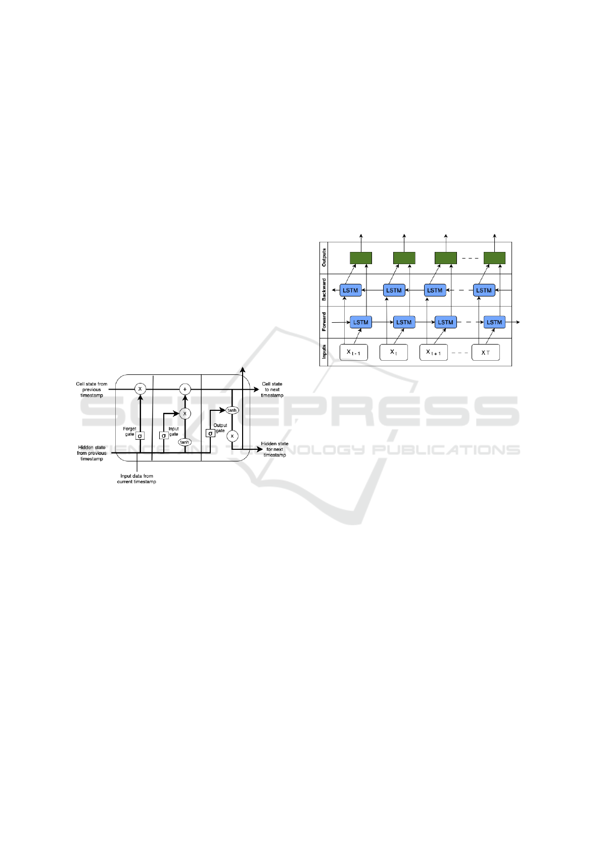
mation within the memory. As shown in Figure 1, an

LSTM memory cell consists of a forget gate, an input

gate, and an output gate.

Figure 1: The structure of an LSTM memory cell.

The forget gate is responsible for deciding which

information from the previous time step should be for-

gotten or retained in the cell’s memory. To make the

decision, the forget gate uses an activation function,

such as sigmoid, which takes both the cell’s old and

new states as input. The input gate decide which new

input data is worth saving in the memory. It utilizes

another activation function, along with weights and

biases, to compute the worthiness of the input data.

The output gate is responsible for determining the

next hidden state of the cell. Here, current states are

processed through another activation function. The

results of the activation function are passed on to the

forget gate of the next cell, which then becomes the

current cell, where the whole process is repeated.

Bi-LSTM is a variation of LSTM (Raihan and

Ahmed, 2023). Figure 2 depicts the architecture of

a Bi-LSTM model. In LSTM, the ﬂow of data and

information is in the forward direction. However,

Bi-LSTM combines two LSTM models, which al-

low data and information to ﬂow in both forward and

backward directions. The forward LSTM processes

the original sequences of data in a forward manner,

while the backward LSTM handles the sequences in a

reversed order. In sequential time series data, under-

standing the context of the data is crucial. Learning

data in both directions helps uncover hidden contex-

tual information within the data (Raihan and Ahmed,

2023). This is why we chose Bi-LSTM for develop-

ing our anomaly detection approach in this paper.

Figure 2: Illustration of how a Bi-LSTM model processes

data in two directions.

4 METHODOLOGY

This section explains the methodology for UoCAD. It

includes an illustration of the overall architecture and

workﬂow in Figure 3. As depicted in the ﬁgure, multi-

variate time series data comes from sensors deployed

within a smart home. UoCAD works in an online

manner to detect contextual anomalies using a slid-

ing window method. Figure 4 shows a small snippet

of the dataset with annotated sliding windows. Be-

fore further explaining the sliding window, we clar-

ify that the term ’instance’ refers to a collection of

data values taken from all of the sensors at a speciﬁc

timestamp. In addition, we use the term ’feature’ to

represent each variable of the multivariate time series.

If we assume that there are a total of ten instances,

and the window size is ﬁve, with every window jump-

ing exactly one instance, there will be a total of six

windows, as shown in Figure 4. Each window con-

tains four overlapping instances from the previous

window and one new instance. Since UoCAD re-

quires a certain number of instances to form a win-

dow, the processing starts when the required amount

of instances has been accumulated.

Whenever a new window of instances is available,

UoCAD goes through an online preprocessing step

where data values of each feature within the window

UoCAD: An Unsupervised Online Contextual Anomaly Detection Approach for Multivariate Time Series from Smart Homes

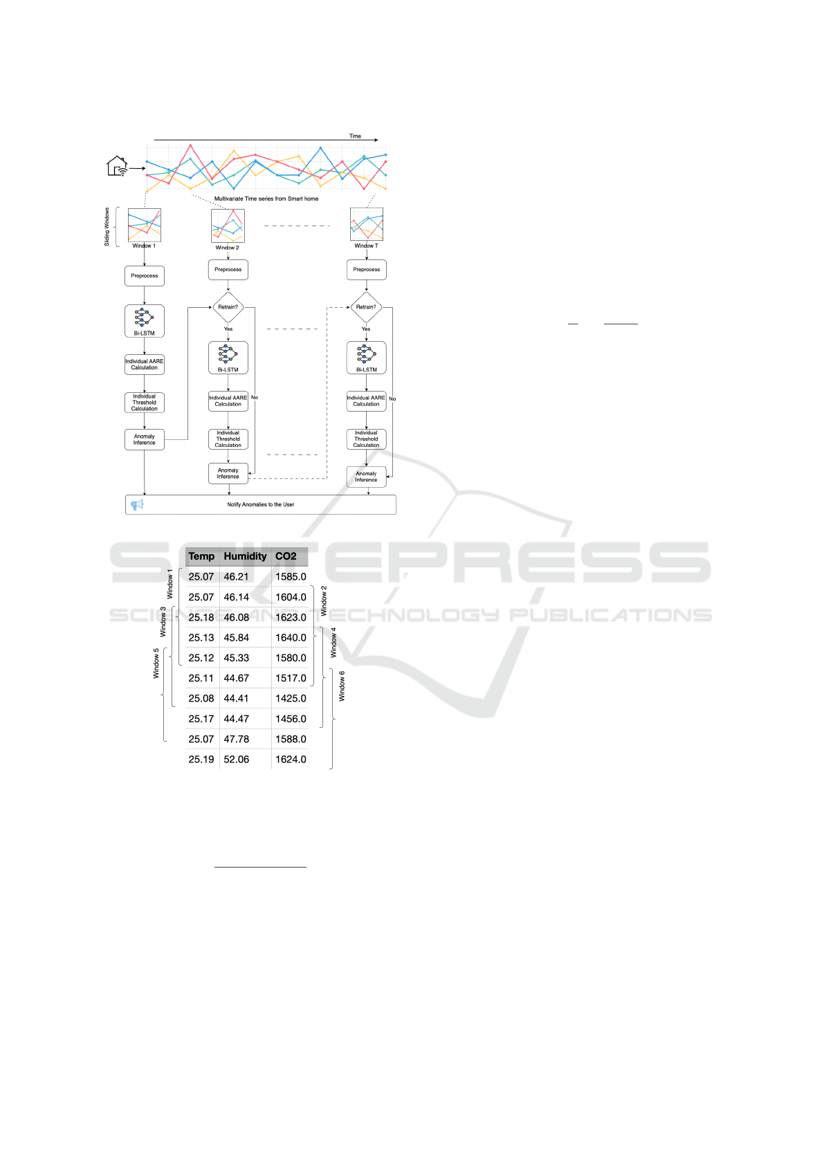
Figure 3: Overall architecture and workﬂow of UoCAD.

Figure 4: Snippet of data with annotated sliding windows.

are normalized to a consistent level using MinMax as

shown in Equation 1, which is a common scaling tech-

nique.

´x =

x − min(x)

max(x) − min(x)

(1)

Here, x is the original value, and ´x is the normalized

value that is scaled to fall within the [0, 1] range. Min-

Max transforms the original values into their equiva-

lent alternatives within the given range but the dis-

tances between values are kept intact. Preprocessing

the data is an important step before feeding it into the

model because well-structured and clean data yields

better results.

This prepares the window for the next step.

As shown in Figure 3, each window is used to train

and retrain a new Bi-LSTM model; however, model

retraining depends on the current model’s prediction

effectiveness. Inspired by the design of RoLA in (Lee

and Lin, 2023b), UoCAD measures the prediction ef-

fectiveness of the current Bi-LSTM model by calcu-

lating an Average Absolute Relative Error (AARE)

value for each feature using Equation 2.

AARE

∑

i=1

− ˆy

| (2)

where M denotes each individual feature, y

repre-

sents the actual value of feature M at timestamp y, ˆy

represents the predicted value of feature M at times-

tamp y, and N is the sliding window size.

In addition, UoCAD does not use a ﬁxed detec-

tion threshold like many previous studies. Instead, it

calculates a dynamic threshold for each feature using

Equation 3.

T hd

= µ

AARE

+ 3 · σ

AARE

(3)

where µ

AARE

is the mean of all historical AARE val-

ues associated with feature M, and σ

AARE

is the cor-

responding standard deviation.

Once the AARE value and threshold are derived

for each feature, UoCAD decides 1) whether re-

training a new Bi-LSTM model is necessary, and

2) whether there is an anomaly or not. To allow

the model to adapt to minor pattern changes in the

time series, UoCAD adopts a double-check approach.

Whenever the AARE value associated with any one

of the features exceeds the corresponding threshold,

UoCAD retrains a new model using the most recent

window, re-predicts the next value of each feature,

and recalculates the corresponding AARE value and

threshold for each feature. If the resulting AARE val-

ues of all the features fall below the corresponding

thresholds, no anomaly is considered as UoCAD con-

siders the deviation to be just a minor pattern change.

However, if any resulting AARE value exceeds the

corresponding threshold, UoCAD further determines

anomalies.

In this paper, we explore two criteria, individ-

ual criterion, and majority criterion, for determining

anomalies. With the individual criterion, if UoCAD

detects that the AARE value associated with any fea-

ture exceeds the corresponding threshold, UoCAD

considers there is an anomaly on that feature at the

moment and notiﬁes the user.

On the other hand, with the majority criterion, if

UoCAD detects that the AARE values associated with

more than half of the features exceeding their corre-

sponding thresholds, UoCAD considers that there is

IoTBDS 2024 - 9th International Conference on Internet of Things, Big Data and Security

anomaly on these features at the moment and notiﬁes

the user.

5 EXPERIMENTS AND RESULTS

This section describes a detailed description of the

experiments conducted to evaluate UoCAD, includ-

ing details about the used dataset and the contextual

anomalies within it.

5.1 Dataset Description

To evaluate the performance of UoCAD, we deployed

an air quality sensor device called the AirThings View

Plus (AirThings, 2024) inside a smart home and uti-

lized the device to collect indoor air quality data.

The devices monitor nine different features: tempera-

ture, particle matter (PM) 10, PM 2.5, volatile organic

compounds (VOC), humidity, carbon dioxide (CO2),

pressure, noise, and light.

To capture the data, both the AirThings View

Plus (AirThings, 2024) and AirThings Hub were

placed inside the kitchen of the smart home. The

AirThings View Plus is connected to a power source

through a USB-C cable and communicates with the

AirThings Hub using SmartLink wireless technology.

The AirThings Hub uses WiFi to transmit live data to

the AirThings cloud. The AirThings cloud provides

access to the data through their dashboard, which not

only offers real-time visualization of the data but also

allows us to download the data. This enables con-

tinuous access to data values from the nine above-

mentioned features. Sensor data readings were taken

at regular intervals of 2.5 minutes. The dataset used

in this study was collected from November 2, 2023,

00:01:54 to November 3, 2023, 23:59:24, consisting

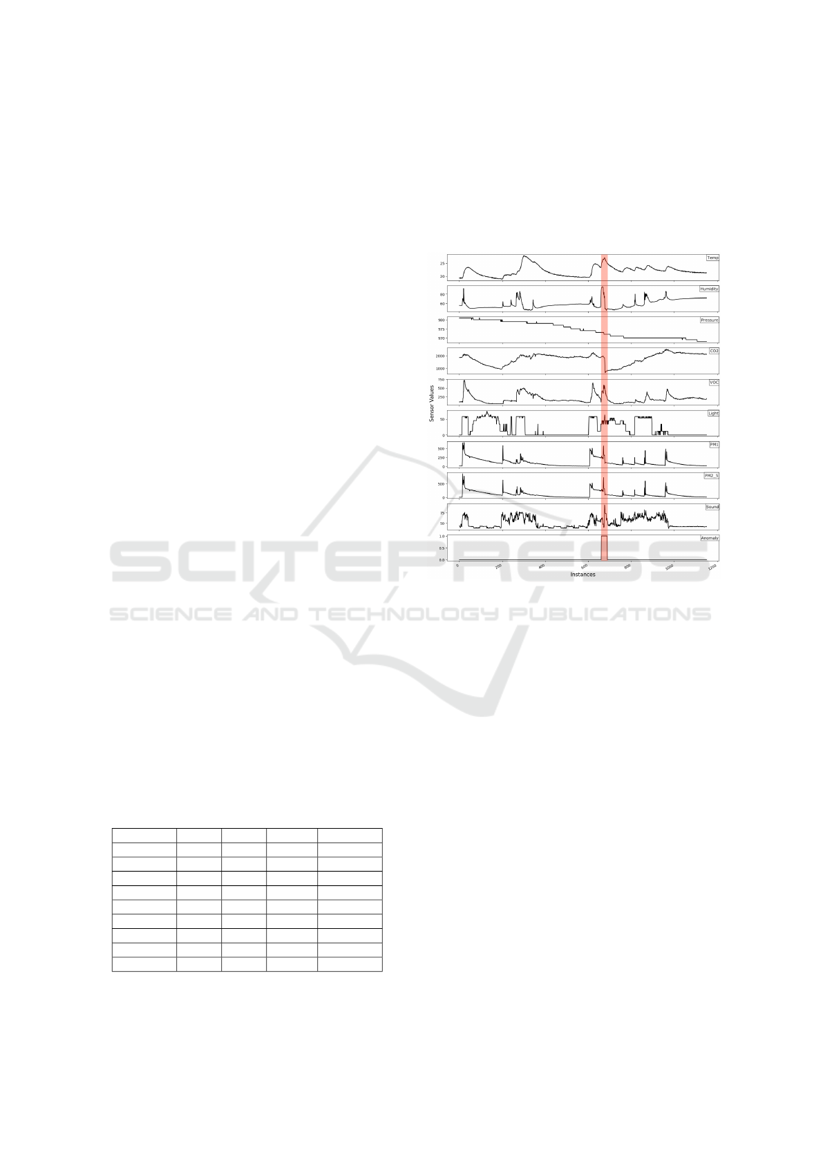
of a total of 1151 instances. Figure 5 shows the visu-

alization of the dataset and highlights the anomalous

region in red. A more detailed introduction to this re-

gion will be provided shortly.

Table 1: Summary of the AirThings dataset.

Feature Min. Max. Avg. Std. Dev.

Temp 18.79 27.89 22.0 1.97

Humidity 44.62 95.76 58.53 9.51

Pressure 968.0 981.0 974.5 4.32

CO2 635 2518 1757.5 434.54

VOC 46 721 188.30 121.65

Light 0 74 21.39 25.01

PM10 1 659 97.95 100.81

PM2.5 1 852 101.19 106.32

Sound 37 94 50.80 12.13

Table 1 shows a summary of the dataset, including

the minimum, maximum, average value, and standard

deviation for each feature. In addition, the dataset

includes timestamps and anomaly labels. All sen-

sor values are represented as real numbers, while the

timestamps are in DateTime format. The anomaly la-

bels are binary, with ’1’ denoting a normal instance

and ’0’ denoting an abnormal instance.

Figure 5: Visualization of the AirThings dataset.

To make the data well-structured and consistent,

some processing was performed on the data. For some

of the sensor values, there was a two-second lag in

sending the data to the cloud. For example, if sen-

sor values for temperature, humidity, CO2, and light

are sent to the cloud at 13:00:00, then the values for

PM2.5, PM10, VOC, and sound are sent to the cloud

at 13:00:02. The reason for this difference is prob-

ably related to the management of data communica-

tion, i.e., sending all of the data to the cloud at the

same time might take more bandwidth and causes de-

lay. Nevertheless, this discrepancy was removed by

setting the timestamp of the said instance to 13:00:01

and merging all nine sensor values to form a single in-

stance. This does not affect the time interval between

two consecutive sensor readings, which remains the

same at 2.5 minutes.

5.2 Contextual Anomaly

Recall that the focus of UoCAD is to detect contex-

tual anomalies. To understand and identify contex-

tual anomalies, it is important to know the activities

and events occurring in the vicinity of the sensors.

UoCAD: An Unsupervised Online Contextual Anomaly Detection Approach for Multivariate Time Series from Smart Homes

In the case of a smart home, if we do not have in-

formation about the actions taking place in the room

and the events causing ﬂuctuations in sensor values,

it is challenging to infer contextual anomalies. Be-

cause of this, as stated earlier, many studies consider

introducing synthetic contexts into their datasets due

to the unavailability of the actual contexts. However,

the dataset used in this study was collected with the

context in mind. Therefore, the labeled contextual

anomaly in this dataset corresponds to a real event that

happened in the room.

In our dataset, there is one labeled contextual

anomaly, spanning 28 instances, as highlighted in

Figure 5. The focus of this dataset is cooking activ-

ity, which has a considerable impact on sensor values.

Several repetitive spikes shown in Figure 5 represent

the cooking activities. Cooking occurs 2-3 times a

day for breakfast, lunch, and dinner, and except for

weekends, the time of cooking is similar across the

days.

The AirThings View Plus device was placed

within a one-meter distance from the stove to record

all cooking activities. Cooking causes an increase in

temperature, PM2.5, PM10, and VOC, and a decrease

in CO2. The contextual anomaly comes from an ’un-

intended cooking’ activity. The scenario is as if some-

one left a pot with food on the stove and forgot to

turn off the stove. To create this contextual anomaly,

some vegetables were put in a pot with some water

and placed on a turned-on stove for one hour. After

the water evaporated, the vegetables started to burn,

which generated a lot of smoke. This caused ﬂuctu-

ations in humidity, PM2.5, PM10, CO2, VOC, and

sound, the last of which was due to the triggering of

the smoke alarm.

5.3 Experimental Setup

All the experiments conducted for this study were per-

formed using Google Colab, which provides 12 GB

of RAM, 107 GB of disk space, and support of Cloud

TPU v5e. The code implementation was carried out

using the end-to-end machine learning library Ten-

sorFlow (Abadi et al., 2016) and neural network li-

brary Keras (Chollet et al., 2015). Both libraries are

Python-based and facilitate a wide range of machine

learning and deep learning tasks.

Table 2 lists the parameter settings of the Bi-

LSTM model used in UoCAD. The model employs

two LSTM layers: One is a forward, and the other is a

backward layer. Both layers utilize a total of 32 neu-

rons. The model is run for up to 50 epochs for each

sliding window that requires retraining. Early stop-

ping is used to avoid wasting unnecessary time when

the model does not learn new knowledge. The com-

monly used activation function, LeakyReLU, and the

loss function, Mean Absolute Error, are used along

with a learning rate of 0.01 and a dropout rate of 0.2.

The validation split within the model is set to 0.25,

and the batch size is set to 16.

Table 2: Bi-LSTM hyperparameters for UoCAD.

Hidden Layers

2 (forward and backward)

Number of Neurons 32

Number of Epochs 50 (with early stopping)

Learning Rate 0.01

Dropout Rate 0.2

Activation Function LeakyReLU

Loss Function Mean Absolute Error

Validation Split 0.25

Batch Size 16

To evaluate how different sliding window settings

affect the performance of UoCAD, we considered the

following eight different window sizes: 6, 12, 24, 48,

73, 96, 120, and 144. These window sizes were se-

lected based on data intervals in time series, namely

2.5 minutes. The window sizes of 6, 12, 24, 48, 72,

96, 120, 144 correspond to 15, 30, 60, 120, 180, 240,

300, 360 minutes, respectively. Taking into account

both the individual criterion and the majority crite-

rion, there are 16 (=2*8) combinations in total. In the

rest of the paper, ’Individual-6’ refers to UoCAD uti-

lizing the individual criterion and a window size of

6, ’Individual-12’ refers to UoCAD utilizing the in-

dividual criterion and a window size of 12, and so

on. Similarly, ’Majority-6’ refers to UoCAD utiliz-

ing the majority criterion and the window size of 6,

’Majority-12’ refers to UoCAD utilizing the majority

criterion and the window size of 12, and so on. When

each of these combinations were evaluated, they all

had the same hyperparameter setting, as shown in Ta-

ble 2.

5.4 Performance Metrics

Key performance metrics used to evaluate the model

results are Precision, Recall, and F1-score. Precision

and recall are calculated using the formulas given in

Equations 4 and 5, respectively. Precision is the ra-

tio between true positives and all predicted positives,

and it indicates the proportion of correctly identiﬁed

anomalies by the model. Recall is the ratio of true

positives to all actual positives. A higher recall means

that the model is better at identifying all positive in-

stances. F1-score, as given in Equation 6, is a metric

that combines both precision and recall to provide a

single measure of the performance of a model.

IoTBDS 2024 - 9th International Conference on Internet of Things, Big Data and Security

Precision =

TruePositives

TruePositives + FalsePositives

(4)

Recall =

TruePositives

TruePositives + FalseNegatives

(5)

F1-score = 2 ·

Precision · Recall

Precision + Recall

(6)

To calculate these metrics, we combine the ap-

proaches used by (Lee et al., 2021) and (Ren et al.,

2019). To be more speciﬁc, if an anomaly that oc-

curs from time point a to time point e can be detected

within the time period from time point a − c to time

point e + c, where c is a small number of time points,

we say the anomaly is successfully detected, as the

anomaly notiﬁcation will alert the user and prompt

the necessary response. This period is called a valid

detection period. According to (Ren et al., 2019), it is

suggested to set c to 7 for minutely intervals and 3 for

hourly intervals. In our case, with the time interval of

2.5 minutes, we set c equal to 7. For example, if an

anomaly starts at time point 30 and ends at time point

60, then the valid detection period will start at time

point 23 and end at time point 67.

In addition, we evaluated the time consumption

of UoCAD in determining the anomalousness of each

instance in two situations: one when a new model re-

training is required and another when a new model

retraining is not required.

5.5 Results and Discussion

In this section, we provide the results of the experi-

ments performed for this study. Tables 3 presents the

detection results of UoCAD across different window

size settings and the two different criteria (i.e., the 16

above-mentioned combinations).

When UoCAD adopted the individual criterion,

combinations of Individual-12 and Individual-24 led

to the best F1-score of 1.0. On the other hand, with

the majority criterion, Majority-48 led to the best F1-

score of 1.0. Four features repeatedly contributed to

the anomaly detection across all the window sizes,

i.e., Temp, Humidity, CO2, and VOC. From a sim-

plistic point of view, it makes sense because these

features are known to be affected by cooking/burning

activities.

Figure 6 further presents the anomaly detection re-

sults of UoCAD. The region highlighted in red repre-

sents the contextual anomaly and the 16 line charts at

the bottom represent the detected anomalies by Uo-

CAD with the 16 different combinations. Individual-

12, Individual-24, and Majority-48 are considered

best since these are the only combinations that not

only enabled UoCAD to detect the anomalous region

but also reported no false positives. However, if we

look closely at their detected anomalies, we can see

that UoCAD with Individual-12 detected anomalies

at the very start of the anomalous region. This means

that this decision was made based on the previous 12

instances which were not anomalous.

However, with Individual-24, UoCAD reported

two occurrences of anomalies, both at the start and

end of the anomalous region. We consider Individual-

24 to be a better setting because the sensor values start

to rise around the middle of the anomalous region,

which means that anomalies reported by Individual-

12 might be coincidental. On the other hand, with

Individual-24, UoCAD detected anomalies at the end

of the anomalous region, which means this decision

was made based on the previous 24 anomalous in-

stances.

Individual-144, Majority-12, Majority-24, and

Majority-144 were the cases that led to the worst re-

sults, as they could not detect any anomalous instance.

That is why their F1-scores are all zero. Hence, we

can consider 120 as the maximum window size that

can detect some of the anomalous instances.

Table 4 shows time performance of UoCAD under

different sliding window sizes. Since the training and

prediction times for both the individual criterion and

the majority criterion are almost the same, we do not

present their time analysis separately. Time analysis

is conducted in this paper because, for any real-time

anomaly detection approach, quickly processing and

identifying anomalies in the current sliding window

is very important. The approach should be ready to

receive and process the next sliding window within

the given time, which is 2.5 minutes in our case.

In Table 4, the ’Detection Time with Training

(seconds)’ column shows the time required by Uo-

CAD to train a new model, calculate AAREs and

thresholds, predict the next instance, and anomaly in-

ference. On the other hand, the ’Detection Time with-

out Training (seconds)’ column shows the time re-

quired by UoCAD to calculate AAREs and thresh-

olds, predict the next instance, and anomaly infer-

ences. The ’Retrain count’ column, as the name sug-

gests, represents the total number of model retraining

during the processing of all the sliding windows of

the dataset. The last column refers to the number of

instances processed by UoCAD before the ﬁrst model

retraining is performed.

When UoCAD utilizes the window size of 24, it

spends the shortest time, i.e., 7.98 seconds, to deter-

mine whether or not the upcoming instance is anoma-

lous when model retraining is required. Furthermore,

the index of the ﬁrst retrain is 670 when UoCAD uti-

UoCAD: An Unsupervised Online Contextual Anomaly Detection Approach for Multivariate Time Series from Smart Homes

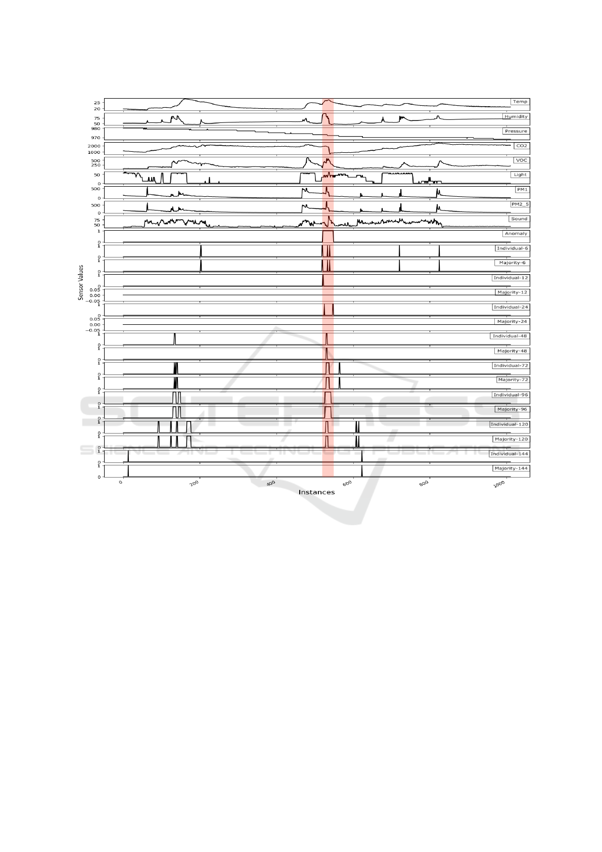
Figure 6: Anomaly detection results of UoCAD in different scenarios.

lizes this window size, which means that UoCAD did

not make any false positive before the anomalous re-

gion.

With the window size of 12, UoCAD took the least

amount of time to process all windows (i.e., 5.9 min-

utes); however, both the average detection time and

the number of true negatives are worse than those

achieved with the window size of 24.

The best retrain count is seen with the window

size of 144, i.e., 6, but UoCAD was unable to detect

any anomalous instance in this case. Similarly, the

window size of 6 led to the best detection time; how-

ever, it resulted in the highest retrain count, which was

caused by multiple anomalies suggested by UoCAD.

Lastly, the window sizes of 6 and 12 led to higher

average anomaly detection time (which includes the

time for model retraining) as compared to other win-

dow sizes which have a larger number of instances

per window to process. One possible reason for this is

that the training time is largely dependent on the num-

ber of epochs executed during each retrain. Since the

early stopping option is used, the epoch count varies

based on model learning. On average, the model was

run for 22-25 epochs for the window sizes 6 and 12,

as compared to other widow sizes which took 15-18

epochs.

6 CONCLUSIONS AND FUTURE

WORK

In this study, we have proposed UoCAD for detect-

ing contextual anomalies in smart-home time series in

an online manner, based on Bi-LSTM and a sliding-

window approach. The key strength of UoCAD lies

IoTBDS 2024 - 9th International Conference on Internet of Things, Big Data and Security

Table 3: Detection performance of UoCAD in different scenarios.

Combination Precision Recall F1-score Detected Features

Individual-6 0.84 1.0 0.91 CO2, Temp, Humidity, VOC

Individual-12 1.0 1.0 1.0 CO2, Temp, Pressure

Individual-24 1.0 1.0 1.0 Temp, Humidity, VOC

Individual-48 0.86 1.0 0.92 Temp, Humidity, CO2, VOC

Individual-72 0.86 1.0 0.92 Temp, Humidity, CO2, VOC, PM2.5, PM10

Individual-96 0.75 1.0 0.86 Temp, Humidity, CO2, VOC

Individual-120 0.66 1.0 0.80 Humidity CO2, VOC

Individual-144 0 0 0 Temp, Humidity, CO2

Majority-6 0.84 1.0 0.91 CO2, Temp, Humidity, VOC

Majority-12 0 0 0 CO2, Temp, Pressure

Majority-24 0 0 0 Temp, Humidity, VOC

Majority-48 1.0 1.0 1.0 Temp, Humidity, CO2, VOC

Majority-72 0.86 1.0 0.92 Temp, Humidity, CO2, VOC, PM2.5, PM10

Majority-96 0.75 1.0 0.86 Temp, Humidity, CO2, VOC

Majority-120 0.66 1.0 0.80 Humidity CO2, VOC

Majority-144 0 0 0 Temp, Humidity, CO2

Table 4: Time performance of UoCAD for both the individual and majority criteria.

Combinations

Windows

Processed

Detection Time with

Training (seconds)

Detection Time without

Training (seconds)

Retrain

Count

Total Time

(minutes)

Index of

First

Retrain

Average Std. Dev. Average Std. Dev.

6 1147 8.35 0.95 0.20 0.12 43 12.2 12

12 1141 9.30 2.05 0.20 0.10 10 5.94 654

24 1129 7.98 0.95 0.22 0.14 23 8.2 670

48 1105 8.91 0.95 0.28 0.13 19 7.74 34

72 1081 10.58 1.46 0.42 0.46 21 8.30 207

96 1057 11.98 1.59 0.47 0.63 42 12.9 179

120 1033 11.53 1.06 0.61 0.70 24 10.24 117

144 1009 14.02 1.58 0.60 0.50 6 7.01 15

in its ability to predict the upcoming values for each

feature and calculate the corresponding prediction er-

ror values and detection thresholds, allowing for ei-

ther adapting to minor pattern changes or identify-

ing anomalies. Furthermore, we have explored two

distinct criteria, the individual and majority criteria,

for anomaly detection. The individual criterion ﬂags

an anomaly if any feature is identiﬁed as anomalous,

while the majority criterion triggers an anomaly when

more than half of the features exhibit anomalous be-

havior.

The evaluation of UoCAD was performed us-

ing an air quality sensor dataset collected from a

smart home. A total of 16 combination scenarios

were used to assess the detection performance of Uo-

CAD. UoCAD performed best with the Individual-12,

Individual-24, and Majority-48 combinations because

they led to high Precision, Recall, and F1-score with

zero false positives. We also highlighted important

features that contributed to contextual anomaly detec-

tion. In addition, we assessed the time performance

of UoCAD. The results suggest Individual-24 outper-

forms all the other scenarios.

In the future, we will extend our proposed

methodology to make it more generalized for differ-

ent types of anomalies, including point anomalies and

sequence anomalies. Furthermore, we would like to

enhance the performance of UoCAD by further adopt-

ing the concept of incremental learning so that the

model will not be retrained from scratch.

REFERENCES

Abadi, M., Agarwal, A., Barham, P., Brevdo, E., Chen, Z.,

Citro, C., Corrado, G. S., Davis, A., Dean, J., Devin,

M., et al. (2016). Tensorﬂow: Large-scale machine

learning on heterogeneous distributed systems. arXiv

preprint arXiv:1603.04467.

AirThings (2024). View plus - smart indoor air quality mon-

itor.

UoCAD: An Unsupervised Online Contextual Anomaly Detection Approach for Multivariate Time Series from Smart Homes

Belay, M. A., Blakseth, S. S., Rasheed, A., and Salvo Rossi,

P. (2023). Unsupervised anomaly detection for iot-

based multivariate time series: Existing solutions, per-

formance analysis and future directions. Sensors,

23(5):2844.

Bhoomika, A., Chitta, S. N. S., Laxmisetti, K., and Sirisha,

B. (2023). Time series forecasting and point anomaly

detection of sensor signals using lstm neural network

architectures. In 2023 10th International Conference

on Computing for Sustainable Global Development

(INDIACom), pages 1257–1262.

Calikus, E., Nowaczyk, S., Bouguelia, M.-R., and Dikmen,

O. (2022). Wisdom of the contexts: active ensemble

learning for contextual anomaly detection. Data Min-

ing and Knowledge Discovery, 36(6):2410–2458.

Carmona, C. U., Aubet, F.-X., Flunkert, V., and Gasthaus, J.

(2021). Neural contextual anomaly detection for time

series. arXiv preprint arXiv:2107.07702.

Chevrot, A., Vernotte, A., and Legeard, B. (2022). Cae:

Contextual auto-encoder for multivariate time-series

anomaly detection in air transportation. Computers &

Security, 116:102652.

Chollet, F. et al. (2015). Keras: deep learning library for

theano and tensorﬂow. 2015.

Dai, W., Liu, X., Heller, A., and Nielsen, P. S. (2021). Smart

meter data anomaly detection using variational recur-

rent autoencoders with attention. In International

Conference on Intelligent Technologies and Applica-

tions, pages 311–324. Springer.

Golmohammadi, K. and Zaiane, O. R. (2015). Time se-

ries contextual anomaly detection for detecting mar-

ket manipulation in stock market. In 2015 IEEE in-

ternational conference on data science and advanced

analytics (DSAA), pages 1–10. IEEE.

Hayes, M. A. and Capretz, M. A. (2015). Contextual

anomaly detection framework for big sensor data.

Journal of Big Data, 2(1):1–22.

Hela, S., Amel, B., and Badran, R. (2018). Early anomaly

detection in smart home: A causal association rule-

based approach. Artiﬁcial intelligence in medicine,

91:57–71.

Kosek, A. M. (2016). Contextual anomaly detection for

cyber-physical security in smart grids based on an ar-

tiﬁcial neural network model. In 2016 Joint Workshop

on Cyber-Physical Security and Resilience in Smart

Grids (CPSR-SG), pages 1–6. IEEE.

Lee, M.-C. and Lin, J.-C. (2023a). Repad2: Real-time,

lightweight, and adaptive anomaly detection for open-

ended time series. arXiv preprint arXiv:2303.00409.

Lee, M.-C. and Lin, J.-C. (2023b). Rola: A real-time online

lightweight anomaly detection system for multivariate

time series. arXiv preprint arXiv:2305.16509.

Lee, M.-C., Lin, J.-C., and Gran, E. G. (2021). Salad:

Self-adaptive lightweight anomaly detection for real-

time recurrent time series. In 2021 IEEE 45th An-

nual Computers, Software, and Applications Confer-

ence (COMPSAC), pages 344–349. IEEE.

Li, G. and Jung, J. J. (2023). Deep learning for anomaly de-

tection in multivariate time series: Approaches, appli-

cations, and challenges. Information Fusion, 91:93–

102.

Matar, M., Xia, T., Huguenard, K., Huston, D., and Wshah,

S. (2023). Multi-head attention based bi-lstm for

anomaly detection in multivariate time-series of wsn.

In 2023 IEEE 5th International Conference on Artiﬁ-

cial Intelligence Circuits and Systems (AICAS), pages

1–5.

Nizam, H., Zafar, S., Lv, Z., Wang, F., and Hu, X. (2022).

Real-time deep anomaly detection framework for mul-

tivariate time-series data in industrial iot. IEEE Sen-

sors Journal, 22(23):22836–22849.

Pasini, K., Khouadjia, M., Sam

e, A., Tr

epanier, M., and

Oukhellou, L. (2022). Contextual anomaly detection

on time series: A case study of metro ridership analy-

sis. Neural Computing and Applications, pages 1–25.

Raihan, A. S. and Ahmed, I. (2023). A bi-lstm au-

toencoder framework for anomaly detection–a case

study of a wind power dataset. arXiv preprint

arXiv:2303.09703.

Ren, H., Xu, B., Wang, Y., Yi, C., Huang, C., Kou, X., Xing,

T., Yang, M., Tong, J., and Zhang, Q. (2019). Time-

series anomaly detection service at microsoft. In Pro-

ceedings of the 25th ACM SIGKDD international con-

ference on knowledge discovery & data mining, pages

3009–3017.

Velasco-Gallego, C. and Lazakis, I. (2022). Radis: A real-

time anomaly detection intelligent system for fault di-

agnosis of marine machinery. Expert Systems with Ap-

plications, 204:117634.

Wei, Y., Jang-Jaccard, J., Xu, W., Sabrina, F., Camtepe,

S., and Boulic, M. (2023). Lstm-autoencoder-based

anomaly detection for indoor air quality time-series

data. IEEE Sensors Journal, 23(4):3787–3800.

Yu, X., Lu, H., Yang, X., Chen, Y., Song, H., Li, J., and Shi,

W. (2020). An adaptive method based on contextual

anomaly detection in internet of things through wire-

less sensor networks. International Journal of Dis-

tributed Sensor Networks, 16(5):1550147720920478.

IoTBDS 2024 - 9th International Conference on Internet of Things, Big Data and Security