Evaluating the Impact of Generative Adversarial Network in Android

Malware Detection

Fabio Martinelli

, Francesco Mercaldo

2,1

and Antonella Santone

Institute for Informatics and Telematics, National Research Council of Italy (CNR), Pisa, Italy

Department of Medicine and Health Sciences “Vincenzo Tiberio”, University of Molise, Campobasso, Italy

Keywords:

Malware, Deep Learning, GAN, Android, Security.

Abstract:

The recent development of Generative Adversarial Networks demonstrated a great ability to generate images

indistinguishable from real images, leading the academic and industrial community to pose the problem of

recognizing a fake image from a real one. This aspect is really crucial, as a matter of fact, images are used in

many ﬁelds, from video surveillance but also to cybersecurity, in particular in malware detection, where the

scientiﬁc community has recently proposed a plethora of approaches aimed at identifying malware applications

previously converted into images. In fact, in the context of malware detection, using a Generative Adversarial

Network it might be possible to generate examples of malware applications capable of evading detection

by antimalware (and also able to generate new malware variants). In this paper, we propose a method to

evaluate whether the images produced by a Generative Adversarial Network, obtained starting from a dataset of

malicious Android applications, can be distinguishable from images obtained from real malware applications.

Once the images are generated, we train several supervised machine learning models to understand if the

classiﬁers are able to discriminate between real malicious applications and generated malicious applications.

We perform experiments with the Deep Convolutional Generative Adversarial Network, a type of Generative

Adversarial Network, showing that currently the images generated, although indistinguishable to the human

eye, are correctly identiﬁed by a classiﬁer with an F-Measure greater than 0.8. Although most of the generated

images are correctly identiﬁed as fake, some of them are not recognized as such, they are therefore considered

images generated by real applications.

1 INTRODUCTION AND

RELATED WORK

Generative Adversarial Networks (GANs) are a class

of neural networks utilized in unsupervised machine

learning. They consist of two opposing components:

a generator, responsible for producing synthetic data,

and a discriminator (or cost network), tasked with dis-

cerning real data from the generated fakes. The gener-

ator and discriminator engage in a competition where

the generator aims to deceive the discriminator with

realistic data, while the discriminator seeks to iden-

tify the real from the fake.

This adversarial interplay fosters the learning of

a generator that can create remarkably authentic data

samples. Once the GAN is trained on a speciﬁc

dataset, it becomes capable of tasks like future pre-

diction or image generation with high ﬁdelity. How-

ever, GANs ﬁnd broader applications across vari-

ous domains, including style transfer, data augmenta-

tion, text generation, and video synthesis(Goodfellow

et al., 2020).

Recently, there has been a growing interest in

the application of GANs in the ﬁeld of cybersecu-

rity. The rationale behind this interest is quite appar-

ent: by generating deceptive data that closely resem-

bles authentic information, GANs offer a way to ex-

ploit vulnerabilities in security systems. This process

is known as ”evasion,” wherein the security system

fails to detect the falsiﬁed data, leading to a success-

ful breach. Biometric authentication systems, among

others, can be particularly susceptible to such attacks.

The danger posed by adversarial technologies pri-

marily lies in their ability to bypass alarms and ac-

cess control mechanisms that have been trained using

available data. Consequently, they pose a signiﬁcant

threat to defensive systems. However, it’s worth not-

ing that these very same adversarial technologies can

also be used as a defensive tool. By leveraging GANs

and related techniques, security experts can design

590

Martinelli, F., Mercaldo, F. and Santone, A.

Evaluating the Impact of Generative Adversarial Network in Android Malware Detection.

DOI: 10.5220/0012699000003687

Paper published under CC license (CC BY-NC-ND 4.0)

In Proceedings of the 19th International Conference on Evaluation of Novel Approaches to Software Engineering (ENASE 2024), pages 590-597

ISBN: 978-989-758-696-5; ISSN: 2184-4895

anomaly detection and authentication systems that are

more resilient against such attacks. In this context,

GANs serve as a valuable asset in fortifying cyberse-

curity measures.

Lately, with the advancement of deep learning and

its capacity to construct models proﬁcient in image-

related tasks (Mercaldo et al., 2022; Huang et al.,

2024a; Huang et al., 2023; Zhou et al., 2023; Huang

et al., 2021), various approaches have emerged to de-

tect malware using deep learning techniques. These

methodologies leverage the power of deep learning

to achieve effective classiﬁcation performance (Sun

et al., 2021; Mercaldo et al., 2021; Huang et al.,

2024b), especially when dealing with image-based

data in the context of malware detection(Iadarola

et al., 2021).

Starting from these considerations, in this paper

we propose a method aimed to understand whether

GANs can represent a threat to image-based malware

detection. In particular, we consider a Deep Convolu-

tional Generative Adversarial Network (DCGAN) to

generate a set of images starting from a dataset of im-

ages obtained from Android malware. To the best of

the author’s knowledge, this paper represents the ﬁrst

attempt to generate images related to Android mal-

ware. As a matter of fact, only the paper published by

Nguyen et al.(Nguyen et al., 2023) proposes the eval-

uation of malware images generated by a GAN, but

relating to PC malware and not to mobile ones. With

the aim to evaluate the quality of the fake images, we

build several machine learning models aimed to dis-

criminate between real and fake images.

The paper proceeds as follows: in Section 2 we

describe the method we designed and implemented to

understand whether DCGAN is able to generate im-

ages related to Android malware applications that are

indistinguishable from the real ones; the results of the

experimental analysis are shown in Section 3 and, ﬁ-

nally, conclusion and future works are drawn in the

last section.

2 THE METHOD

In this section, we introduce our devised method to

accomplish two objectives: (i) generating images as-

sociated with Android malware applications and (ii)

distinguishing these synthetic images from images

obtained from real-world Android malware instances.

To generate an image from an application, we

have developed a Python script that focuses on ex-

tracting byte values from a binary executable and sub-

sequently creating the corresponding grayscale im-

age.

Figure 1 shows the image generation workﬂow.

To transform a binary into an image, we inter-

pret the sequence of bytes (Bit Vectors in Figure 1)

that represents the binary as the bytes of a grayscale

PNG image (Greyscale Pixel in Figure 1). For this

conversion, we adopt a predetermined width of 256

and a variable length based on the size of the binary.

To achieve this, we have designed a script capable

of encoding any binary ﬁle into a lossless PNG for-

mat(Mercaldo and Santone, 2020).

In essence, the script operates through the follow-

ing steps:

• the binary ﬁle’s individual bytes are converted

into numerical values (ranging from 0 to 255),

which will subsequently determine the pixel

color(Greyscale Pixel in Figure 1);

• each byte corresponds to a grayscale pixel in the

resultant PNG image (Application Image in Fig-

ure 1).

After obtaining the images from real-world An-

droid applications, the subsequent step in the pro-

posed method involves employing DCGAN to gen-

erate fake images associated with Android applica-

tions: this second step related to the proposed method

is shown in Figure 2.

In every GAN, there is a minimum of one gen-

erator (Generator in Figure 2) and one discrimina-

tor (Discriminator in Figure 2). As the generator and

discriminator engage in their adversarial competition,

the generator reﬁnes its capacity to produce images

that closely align with the distribution of the training

data, thanks to the feedback received from the dis-

criminator.

The DCGAN introduced a GAN architecture that

utilizes CNNs to deﬁne the discriminator and genera-

tor.

DCGAN offers several architectural guidelines

aimed at improving training stability(Radford et al.,

2015):

1. substituting pooling layers with strided convolu-

tions in the discriminator and fractional-strided

convolutions in the generator;

2. incorporating batch normalization (batchnorm) in

both the generator and discriminator;

3. removing fully connected hidden layers in deeper

architectures;

4. employing ReLU activation for all generator lay-

ers except the output, which utilizes Tanh;

5. employing LeakyReLU activation in all discrimi-

nator layers.

Evaluating the Impact of Generative Adversarial Network in Android Malware Detection

591

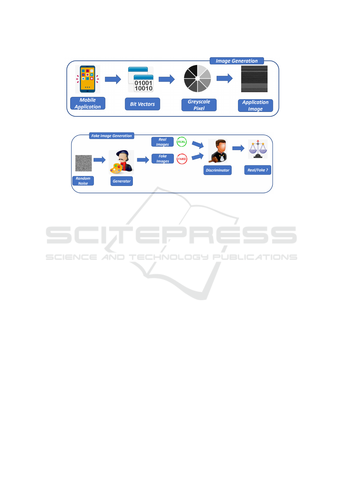
Figure 1: The Image Generation step.

Figure 2: The Fake Image Generation step.

In DCGAN, we make use of batch normalization

(batchnorm) in both the generator and the discrimina-

tor to enhance the stability of GAN training. Batch-

norm operates by standardizing the input layer, ensur-

ing it has a mean of zero and a variance of one. Typi-

cally, batchnorm is inserted after the hidden layer and

before the activation layer.

Within the DCGAN generator and discriminator,

four frequently utilized activation functions are: sig-

moid, tanh, ReLU, and LeakyReLU.

We conduct the training of the generator and dis-

criminator networks concurrently.

The initial stage involves preparing the data for

training. In the case of training a DCGAN, there is no

need to divide the dataset into training, validation, and

testing sets since we are not employing the generator

model for a classiﬁcation task. A set of images ob-

tained from real-world Android malware are obtained

with the procedure shown in Figure 1.

The generator necessitates input images in the for-

mat (60000, 28, 28), which signiﬁes that there are

60,000 training grayscale images with dimensions of

28x28. The loaded data possesses the shape (60000,

28, 28) since it is in grayscale format.

In order to ensure compatibility with the genera-

tor’s ﬁnal layer activation, which uses tanh, we nor-

malize the input images to fall within the range of [-1,

1].

The main objective of the generator is to create

realistic images and trick the discriminator into per-

ceiving them as authentic.

The generator takes random noise as input and

generates an image that closely resembles the train-

ing images. Given that we are generating grayscale

images with dimensions of 28x28, the model archi-

tecture must ensure that the generator’s output has a

shape of 28x28x1.

To accomplish this, the generator undertakes the

following steps:

1. it transforms the 1D random noise (latent vector)

into a 3D shape using the Reshape layer;

2. the generator repeatedly upsamples the noise

by employing the Keras Conv2DTranspose layer

(also known as fractional-strided convolution in

the paper) to achieve the desired output image

size, which, in our case, is a grayscale image with

dimensions of 28x28x1.

The generator comprises several crucial layers

that serve as its fundamental building blocks:

1. Dense (fully connected) layer: primarily used for

reshaping and ﬂattening the noise vector.

2. Conv2DTranspose: employed to upscale the im-

age during the generation process.

3. BatchNormalization: utilized to enhance training

stability, positioned after the convolutional layer

and before the activation function.

Within the generator, ReLU activation is applied

to all layers, excluding the output layer, which utilizes

tanh activation.

ENASE 2024 - 19th International Conference on Evaluation of Novel Approaches to Software Engineering

592

We developed a function for building the gen-

erator model architecture, which model summary is

shown in Table 1.

To construct the generator model, we utilized the

Keras Sequential API. Initially, we added a Dense

layer to facilitate reshaping the input into a 3D for-

mat. It is crucial to specify the input shape within this

initial layer of the model architecture.

Afterward, we incorporated the BatchNormaliza-

tion and ReLU layers into the generator model. Sub-

sequently, we reshaped the preceding layer from 1D

to 3D and performed two upsampling operations us-

ing Conv2DTranspose layers with a stride of 2. This

process enabled us to progress from a 7x7 size to

14x14 and ﬁnally to 28x28, achieving the desired im-

age dimensions.

Following each Conv2DTranspose layer, we in-

cluded a BatchNormalization layer, followed by a

ReLU layer.

Lastly, we utilized a Conv2D layer with a tanh ac-

tivation function.

The generator model comprises a total of

2,343,681 parameters, out of which 2,318,209 are

trainable, while the remaining 25,472 are non-

trainable parameters.

Next, we delve into the implementation of the dis-

criminator model.

The discriminator functions as a simple binary

classiﬁer, responsible for discerning whether an im-

age is real or fake. Its primary goal is to precisely

classify the provided images.

Nevertheless, there are a few differences between

a discriminator and a typical classiﬁer:

1. we employ the LeakyReLU activation function in

the discriminator;

2. the discriminator deals with two categories of in-

put images: real images sourced from the training

dataset labeled as 1, and fake images generated by

the generator labeled as 0.

It is worth noting that the discriminator network is

usually smaller or simpler in comparison to the gener-

ator. This is due to the fact that the discriminator has a

relatively easier task than the generator. In fact, if the

discriminator becomes too powerful, it may impede

the progress and improvement of the generator.

Table 2 shows the model summary related to the

discriminator model.

To build the discriminator model, we will once

more deﬁne a function. The input to the discrimi-

nator comprises either real images (from the training

dataset) or fake images generated by the generator.

These images have a size of 28x28x1, and we pass

the arguments (width, height, and depth) to the func-

tion accordingly.

During the construction of the discriminator

model, we implement Conv2D, BatchNormalization,

and LeakyReLU layers twice for downsampling. Sub-

sequently, we incorporate the Flatten layer and apply

dropout. Finally, in the last layer, we employ the sig-

moid activation function to produce a single value for

binary classiﬁcation.

The discriminator model consists of 213,633 pa-

rameters, with 213,249 being trainable parameters

and 384 being non-trainable parameters.

Calculating the loss is a crucial aspect of training

both the generator and discriminator models in DC-

GAN (or any GAN).

In the context of the DCGAN being considered,

we adopt the modiﬁed minimax loss, which involves

utilizing the binary cross-entropy (BCE) loss func-

tion.

We need to compute two distinct losses: one for

the discriminator and another for the generator.

Concerning the Discriminator Loss, as the dis-

criminator receives two sets of images (real and fake),

we will compute the loss for each group indepen-

dently and then merge them to obtain the overall dis-

criminator loss.

TotalDloss = loss f rom real images +

loss f rom f ake images

With regard to the generator loss, rather than

training G to minimize log(1 − D(G(z)) i.e., to en-

hance the probability of the discriminator, D, cor-

rectly classifying fake images as fake, we focus on

training the generator, G, to maximize this probabil-

ity logD(G(z)) i.e., the probability that D incorrectly

classiﬁes the fake images as real: this the modiﬁed

minimax loss we exploit.

To enhance the probability of the discriminator, D,

correctly classifying fake images as fake, we focus on

training the generator, G, to maximize this probabil-

ity.

The training process consists of 50 epochs.

Once generated the images with the DCGAN, the

last step of the proposed method, shown in Figure 3

is devoted to build models aimed to discriminate be-

tween real and fake images related to Android mal-

ware applications.

As shown in the third step of the proposed method

in Figure 3, to build a model aimed to discern between

generated and real images we need two datasets: the

ﬁrst one is composed by images obtained from An-

droid malware (Real Images in Figure 3), the second

one composed by images generated from the DGCAN

shown in Figure 2 (Generated Images in Figure 3).

The real images are the same we exploited in step two

of the proposed method (i.e., fake image generation

in Figure 2). From the two sets of images, we extract

Evaluating the Impact of Generative Adversarial Network in Android Malware Detection

593

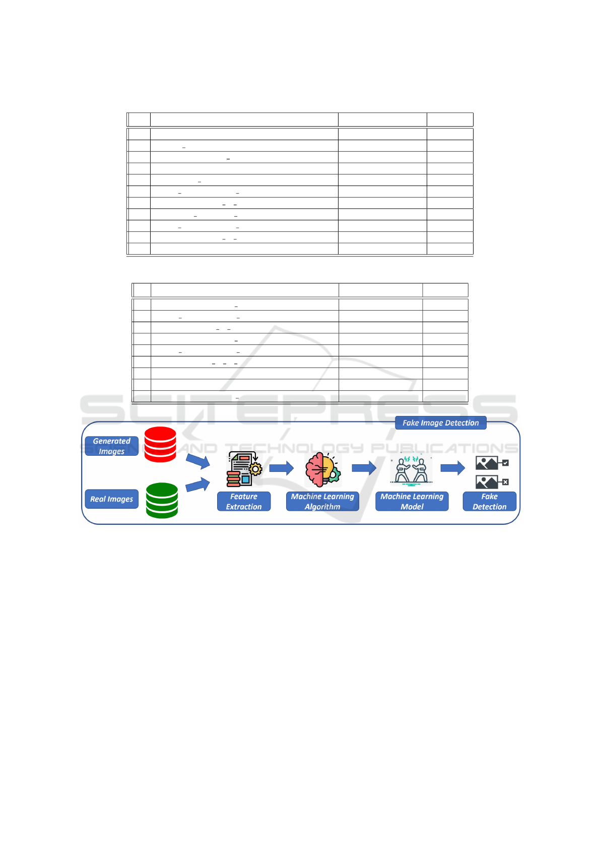
Table 1: Model Generator.

# Layer (type) Output Shape Param #

1 dense (Dense) (None, 12544) 1266944

2 batch normalization (BatchNormalization) (None, 12544) 50176

3 re lu (ReLU) (None, 12544) 0

4 reshape (Reshape) (None, 7, 7, 256) 0

5 conv2d transpose (Conv2DTranspose) (None, 14, 14, 128) 819328

6 batch normalization 1 (BatchNormalization) (None, 14, 14, 128) 512

7 re lu 1 (ReLU) (None, 14, 14, 128) 0

8 conv2d transpose 1 (Conv2DTranspose) (None, 28, 28, 64) 204864

9 batch normalization 2 (BatchNormalization) (None, 28, 28, 64) 256

10 re lu 2 (ReLU) (None, 28, 28, 64) 0

11 conv2d (Conv2D) (None, 28, 28, 1) 1601

Table 2: Model Discriminator.

# Layer (type) Output Shape Param #

1 conv2d 1 (Conv2D) (None, 14, 14, 64) 1664

2 batch normalization 3 (BatchNormalization) (None, 14, 14, 64) 256

3 leaky re lu (LeakyReLU) (None, 14, 14, 64) 0

4 conv2d 2 (Conv2D) (None, 7, 7, 128) 204928

5 batch normalization 4 (BatchNormalization) (None, 7, 7, 128) 512

6 leaky re lu 1 (LeakyReLU) (None, 7, 7, 128) 0

7 ﬂatten (Flatten) (None, 6272) 0

8 dropout (Dropout) (None, 6272) 0

9 dense 1 (Dense) (None, 1) 6273

Figure 3: The Fake Image Detection step.

a set of numeric features using the Simple Color His-

togram Filter. This ﬁlter is designed to compute the

histogram representing the pixel frequencies of each

image. By applying this ﬁlter, we extract 64 numeric

features from each image.

After obtaining the feature set from both the gen-

erated and real images, we use these features as inputs

to a supervised machine learning algorithm. The pur-

pose is to create a model capable of detecting whether

an image is related to a fake or real application (i.e.,

Fake Detection in Figure 3).

Obviously, if the classiﬁers exhibit optimal per-

formance, the generated images will be signiﬁcantly

different from the original ones, otherwise, the ma-

chine learning models will not be able to distinguish

the original images from the generated ones.

Considering that we train the GAN for 50 epochs,

we build a model for each epoch, to understand if

during the various phases of GAN training images

more similar to the originals are gradually generated.

For this reason, considering that for conclusion valid-

ity we exploit four different machine learning algo-

rithms, we consider 50 x 4 = 200 different models in

the experimental analysis.

3 EXPERIMENTAL ANALYSIS

In this section, we present and analyze the results of

the experimental analysis.

ENASE 2024 - 19th International Conference on Evaluation of Novel Approaches to Software Engineering

594

This experiment aims to show whether GANs can

currently be considered a threat to mobile malware

detector deep learning based. For this reason, af-

ter having appropriately generated a series of images

through a DCGAN, we trained several classiﬁers, in

order to understand if they are able to distinguish be-

tween malware and trusted applications. Since the

DCGAN generates a series of images at each epoch,

the performance of the models to distinguish between

images of real applications and fake images is shown,

in order to understand whether as the epochs increase,

given that images are presumably generated more

similar to the real ones, the performance of the classi-

ﬁers (aimed to distinguish between real and fake ap-

plication image) should decrease in case the classiﬁer

fails to correctly identify the real images from the fake

ones.

With the aim to generate images related to An-

droid malware, we exploit a dataset composed by

1000 real-world Android malicious applications (and,

thus, we generated 1000 images related to real-world

applications), among 71 malware families with the

aim to cover the current landscape of Android mal-

ware(Li et al., 2017).

The DCGAN is trained for 50 epochs and each

epoch requires approximately 25 seconds in the ex-

perimental analysis (where we exploited the NVIDIA

T4 Tensor Core GPU). We set the DCGAN to gener-

ate, for each epoch, 1000 fake images.

Four different widespread supervised machine

learning classiﬁers are exploited with the aim to en-

force conclusion validity: J48, SVM, RandomForest,

and Bayes. For each algorithm, we built a model for

each epoch, for a total of 4 models x 50 epochs = 200

different models. Each model is built with the im-

ages obtained from real-world applications and with

the image generated for a certain epoch.

We consider a cross-validation value of k=10 for

model training and testing.

Table 3 shows the experimental analysis results

obtained with the procedure previously explained.

For each epoch, we obtain 1000 images generated

by the GAN, we generate a model (with the 1000 fake

images and the 1000 real ones) and we report for the

model the Precision, Recall, and F-Measure values.

In Table 3 we show the experimental analysis re-

sults: for the reason of space we report the results

related to three epochs: the ﬁrst one (i.e., 0 in the

column Epoch), the middle one (i.e., 25 in the col-

umn Epoch) and the ﬁnal one (i.e., 49 in the column

Epoch), with the aim to understand the general trend.

From the results shown in Table 3 we can ob-

serve that the performances of Precision, Recall, and

F-Measure are quite similar for all the epochs (as

Figure 4: The F-Measure trend, obtained with the J48

model,for the 50 epochs.

Figure 5: The F-Measure trend, obtained with the SVM

model, for the 50 epochs.

a matter of fact, all the values are great than 0.8):

there are no substantial differences between the per-

formances obtained with the models trained with im-

ages obtained with the 25 epoch exams or the 50-th.

This behavior is symptomatic of the fact that the

images generated during the various epochs are no

longer similar to the real ones as the epochs increase.

Furthermore, the values of Precision, Recall, and F-

Measure obtained in any case leave it understood that

a part of fake applications is not correctly recognized

by the various classiﬁers, even when they are gener-

ated in the initial epochs.

To better understand the trend of the classiﬁers

during the several epochs, in Figures 4, 5, 6, 7 we

show the plot of the F-Measure trend for the 50

epochs, respectively, for the J48 model (shown in Fig-

ure 4), the SVM model (shown in Figure 5), the Ran-

domForest one (shown in Figure 6) and the Bayes

model (shown in Figure 7)

From the plots shown in Figures 4, 5, 6, 7 we can

observe that there is no presence of a particular trend,

as a matter of fact, the F-Measure, for all the models

involved in the experiment, is stable to value greater

than 0.8 and this happens regardless of the epoch.

From the machine learning model point of view, as the

epochs increase, images that are more similar to the

real ones are not generated, and this aspect is noted

by F-Measure values which are extremely similar in

all epochs (both the initial and the ﬁnal ones). This

behavior is found in all four models used, so we can

Evaluating the Impact of Generative Adversarial Network in Android Malware Detection

595

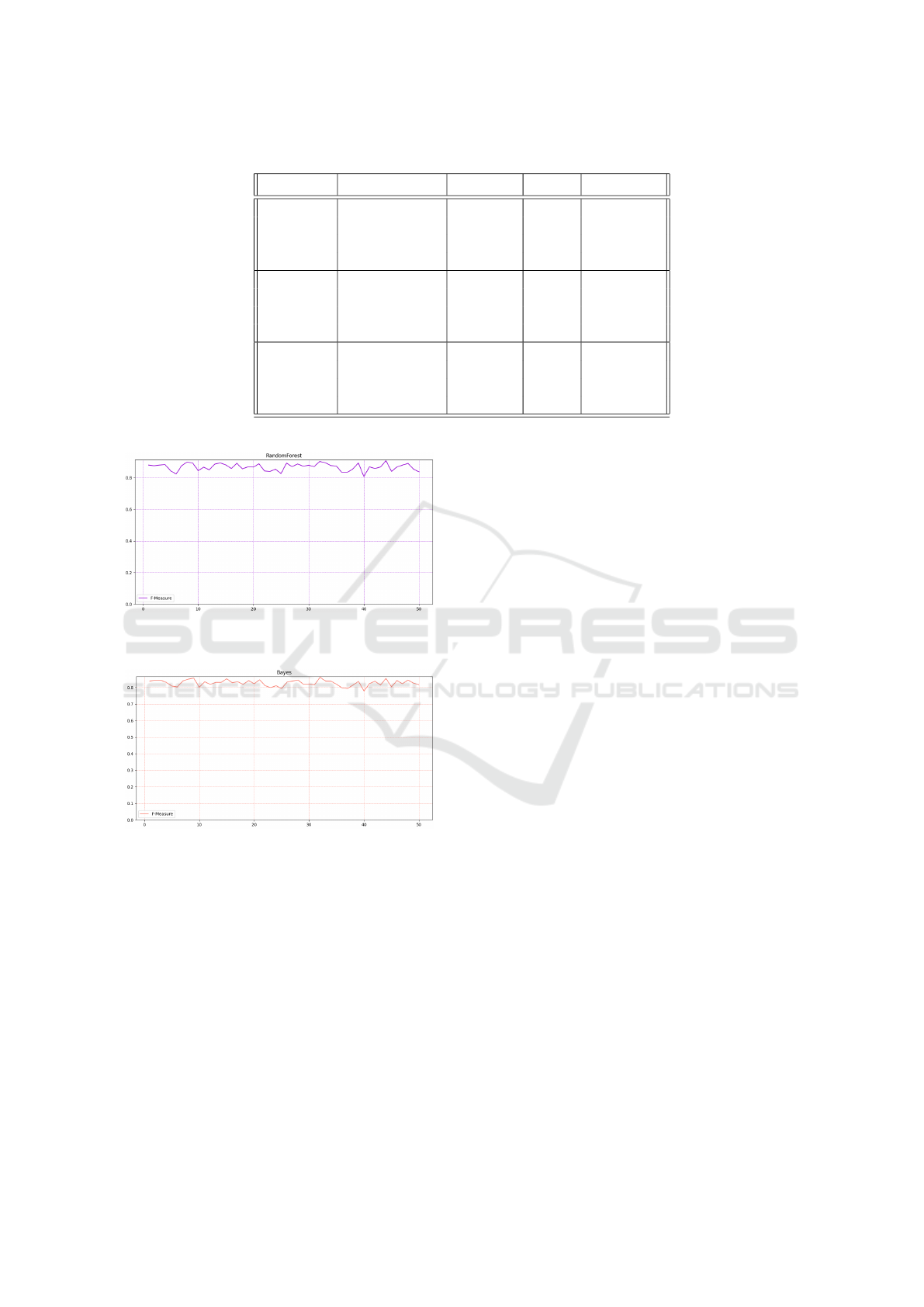
Table 3: Experimental analysis results for the 0, 25, and 49 epochs.

Epoch Algorithm Precision Recall F-Measure

J48 0,877 0,876 0,876

SVM 0,870 0,869 0,869

RandomForest 0,880 0,880 0,880

Bayes 0,839 0,838 0,838

J48 0,892 0,892 0,892

SVM 0,880 0,879 0,879

RandomForest 0,892 0,892 0,892

Bayes 0,832 0,832 0,832

J48 0,835 0,833 0,833

SVM 0,836 0,835 0,835

RandomForest 0,837 0,837 0,837

Bayes 0,816 0,816 0,816

Figure 6: The F-Measure trend, obtained with the Random-

Forest model, for the 50 epochs.

Figure 7: The F-Measure trend, obtained with the Bayes

model, for the 50 epochs.

conclude that this is a general trend and not speciﬁc

to a single classiﬁcation algorithm. For this reason,

it is possible to conclude that, due to the current state

of the art of GANs, they do not currently represent a

threat, as a classiﬁer is able to discriminate between

real images and fake images with quite good perfor-

mances. On the other hand, however, we highlight

that a small percentage of images manage to evade the

controls and, for this reason, to elude detection, and

this aspect in the future could actually pose a threat in

the context of image-based malware detection.

4 CONCLUSION AND FUTURE

WORK

Considering the ability of GANs to generate images

that are indistinguishable from the human eye, the

need arises to understand if they can pose a threat

to image recognition-based systems, including mal-

ware detection that analyzes suitably converted ap-

plications through deep learning in images. We pro-

posed a method aimed to evaluate whether the im-

ages (related to Android malware applications) gener-

ated by a DCGAN can be discriminated by real ones.

Once we generated the images we resort to four dif-

ferent supervised machine-learning algorithms to un-

derstand whether it is possible to build a model aimed

to discriminate between real images (obtained from

Android malware) and fake images. The experimen-

tal analysis showed that all the supervised models

we considered are able to discriminate real images

from fake ones with an F-Measure greater than 0.80,

therefore on the one hand demonstrating that most of

the fake images are recognized, but with the aware-

ness that several images related to Android malware

manage to evade the fake detection models. In fu-

ture work, we plan to consider other kinds of im-

ages obtained, for instance, from the malware sys-

tem call trace and we will evaluate other GANs, for

instance, the conditional generative adversarial net-

work and the cycle-consistent generative adversarial

network to compare the obtained results with the one

shown by the DGCAN exploited in this paper.

ACKNOWLEDGEMENTS

This work has been partially supported by EU DUCA,

EU CyberSecPro, SYNAPSE, PTR 22-24 P2.01 (Cy-

ENASE 2024 - 19th International Conference on Evaluation of Novel Approaches to Software Engineering

596

bersecurity) and SERICS (PE00000014) under the

MUR National Recovery and Resilience Plan funded

by the EU - NextGenerationEU projects.

REFERENCES

Goodfellow, I., Pouget-Abadie, J., Mirza, M., Xu, B.,

Warde-Farley, D., Ozair, S., Courville, A., and Ben-

gio, Y. (2020). Generative adversarial networks. Com-

munications of the ACM, 63(11):139–144.

Huang, P., Li, C., He, P., Xiao, H., Ping, Y., Feng, P., Tian,

S., Chen, H., Mercaldo, F., Santone, A., et al. (2024a).

Mamlformer: Priori-experience guiding transformer

network via manifold adversarial multi-modal learn-

ing for laryngeal histopathological grading. Informa-

tion Fusion, page 102333.

Huang, P., Tan, X., Zhou, X., Liu, S., Mercaldo, F., and

Santone, A. (2021). Fabnet: fusion attention block

and transfer learning for laryngeal cancer tumor grad-

ing in p63 ihc histopathology images. IEEE Journal

of Biomedical and Health Informatics, 26(4):1696–

1707.

Huang, P., Xiao, H., He, P., Li, C., Guo, X., Tian, S.,

Feng, P., Chen, H., Sun, Y., Mercaldo, F., et al.

(2024b). La-vit: A network with transformers con-

strained by learned-parameter-free attention for in-

terpretable grading in a new laryngeal histopathol-

ogy image dataset. IEEE Journal of Biomedical and

Health Informatics.

Huang, P., Zhou, X., He, P., Feng, P., Tian, S., Sun, Y., Mer-

caldo, F., Santone, A., Qin, J., and Xiao, H. (2023).

Interpretable laryngeal tumor grading of histopatho-

logical images via depth domain adaptive network

with integration gradient cam and priori experience-

guided attention. Computers in Biology and Medicine,

154:106447.

Iadarola, G., Martinelli, F., Mercaldo, F., and Santone, A.

(2021). Towards an interpretable deep learning model

for mobile malware detection and family identiﬁca-

tion. Computers & Security, 105:102198.

Li, Y., Jang, J., Hu, X., and Ou, X. (2017). Android mal-

ware clustering through malicious payload mining. In

Research in Attacks, Intrusions, and Defenses: 20th

International Symposium, RAID 2017, Atlanta, GA,

USA, September 18–20, 2017, Proceedings, pages

192–214. Springer.

Mercaldo, F., Martinelli, F., and Santone, A. (2021). A pro-

posal to ensure social distancing with deep learning-

based object detection. In 2021 International Joint

Conference on Neural Networks (IJCNN), pages 1–5.

IEEE.

Mercaldo, F. and Santone, A. (2020). Deep learning

for image-based mobile malware detection. Jour-

nal of Computer Virology and Hacking Techniques,

16(2):157–171.

Mercaldo, F., Zhou, X., Huang, P., Martinelli, F., and San-

tone, A. (2022). Machine learning for uterine cervix

screening. In 2022 IEEE 22nd International Confer-

ence on Bioinformatics and Bioengineering (BIBE),

pages 71–74. IEEE.

Nguyen, H., Di Troia, F., Ishigaki, G., and Stamp, M.

(2023). Generative adversarial networks and image-

based malware classiﬁcation. Journal of Computer

Virology and Hacking Techniques, pages 1–17.

Radford, A., Metz, L., and Chintala, S. (2015). Unsu-

pervised representation learning with deep convolu-

tional generative adversarial networks. arXiv preprint

arXiv:1511.06434.

Sun, X., Li, L., Mercaldo, F., Yang, Y., Santone, A., and

Martinelli, F. (2021). Automated intention mining

with comparatively ﬁne-tuning bert. In Proceedings

of the 2021 5th International Conference on Natu-

ral Language Processing and Information Retrieval,

pages 157–162.

Zhou, X., Tang, C., Huang, P., Tian, S., Mercaldo, F., and

Santone, A. (2023). Asi-dbnet: an adaptive sparse

interactive resnet-vision transformer dual-branch net-

work for the grading of brain cancer histopathological

images. Interdisciplinary Sciences: Computational

Life Sciences, 15(1):15–31.

Evaluating the Impact of Generative Adversarial Network in Android Malware Detection

597