Spatial Performance Indicators to Evaluate Spatiotemporal Traffic
Prediction
Muhammad Farhan Fathurrahman
1,2 a
and Sidharta Gautama
1,2 b
1
Department of Industrial Systems Engineering and Product Design, Ghent University, Ghent, Belgium
2
FlandersMake@UGent-Corelab ISyE, Lommel, Belgium
Keywords: Traffic Prediction, Spatiotemporal Prediction, Spatial Performance Indicators, Global Moran’s I, Geary’s C,
Getis-Ord General G.
Abstract: Traffic prediction is vital for traffic management systems and helps enhance traffic management efficiency
over a traffic network. Recently, spatiotemporal prediction models have been proposed that extend single
traffic node temporal prediction. They employ the spatial context of the combined nodes in the urban network
to improve prediction. However, the key performance indicators (KPI) of these methods are still limited to
accuracy averaged over the full traffic network. They do not yet describe local spatiotemporal behaviour that
can affect the traffic prediction accuracy in the traffic network. In this paper, we explore three spatial KPIs:
Global Moran’s I, Geary’s C, and Getis-Ord General G to evaluate traffic flow prediction for freeway traffic
networks. The study is conducted by evaluating traffic flow prediction results in the PeMSD8 dataset using
spatiotemporal prediction and calculating different KPIs. Several synthetic scenarios based on the prediction
results are created to showcase what the standard KPI cannot distinguish. The Global Moran’s I and Geary’s
C can identify different levels of spatial autocorrelation and the Getis-Ord General G can distinguish spatial
clustering in prediction results. The findings aim to improve the evaluation of different traffic prediction
methods towards a better traffic management system.
1 INTRODUCTION
The prediction of traffic states plays a pivotal role in
enhancing traffic management systems, with
applications ranging from optimizing traffic signal
control to enhancing route planning and guidance.
Traffic predictions in traffic networks are seen as a
challenging problem in time series predictions
because traffic network suffers from a highly
nonlinear dynamic nature, limited resources,
spatiotemporal dependency, and seasonality (Korecki
et al., 2023). Over the past few years, the field of
traffic predictions has witnessed a surge of interest
within the machine learning community. Recently,
spatiotemporal prediction models such as ASTGCN
(Guo et al., 2019) and STSGCN (Song et al., 2020)
have gained popularity due to their ability to utilise
large sets of temporal and spatial data in a network,
which enhances prediction accuracy (Tascikaraoglu,
2018). This ability is crucial in traffic prediction
a
https://orcid.org/0000-0002-4532-1209
b
https://orcid.org/0000-0001-5628-6974
problems where the traffic states are influenced not
only by historical trends over time but also by the
spatial interactions between different locations.
Comparatively, traditional single-node temporal
prediction methods overlook the spatial interactions
and dependencies that exist in traffic networks.
Currently, much of the research in traffic
prediction tends to focus on employing a single
standard key performance indicator (KPI) such as
RMSE, MAE, or MAPE due to the ease of ranking
different techniques. Unfortunately, those KPIs are
limited to the average prediction accuracy for the
entire traffic network even though knowledge
regarding the temporal and spatial contexts is known.
This approach simplifies the evaluation of traffic
prediction, but it may not necessarily reflect the
requirements in actual traffic management systems
which leads to a gap between research findings and
their applicability in the real world. Accuracy is not
the only KPI of a prediction method and accuracy is
156
Fathurrahman, M. and Gautama, S.
Spatial Performance Indicators to Evaluate Spatiotemporal Traffic Prediction.
DOI: 10.5220/0012699200003702
Paper published under CC license (CC BY-NC-ND 4.0)
In Proceedings of the 10th International Conference on Vehicle Technology and Intelligent Transport Systems (VEHITS 2024), pages 156-164
ISBN: 978-989-758-703-0; ISSN: 2184-495X
Proceedings Copyright © 2024 by SCITEPRESS – Science and Technology Publications, Lda.

also not a simple single quantitative metric (Dietel,
2003).
The lack of prediction KPI has been brought up
for discussion in different fields such as randomness
in databases (Fisher et al., 2009), different accuracy
measures in classification problems (Mehdiyev et al.,
2016), evaluation of sparse spatiotemporal point
process (Adepeju et al., 2016), and uncertainty in
spatial forecasting (Wu et al., 2021) but not in traffic
prediction problems. In traffic prediction problems,
the prediction accuracy across different forecast
horizons is sometimes considered but it is limited to
multi-step prediction problems. Evaluating the short-
term and long-term predictions of the spatiotemporal
prediction model provides information on the
robustness and adaptability of the method (Li et al.,
2022) that is crucial in real-world applications but
can’t be evaluated from the current standard KPI.
Prediction accuracy across different forecast horizons
can be considered as an evaluation of temporal
aspects of the spatiotemporal prediction model but the
evaluation of the spatial aspects of the spatiotemporal
method is currently not researched.
In this paper, we will explore several spatial
metrics commonly used in the domain of Geospatial
Information Systems (GIS) such as Global Moran’s I,
Geary’s C, and Getis-Ord General G as spatial KPIs
for traffic prediction problems. We acknowledge that
evaluating both spatial and temporal aspects holds
equal significance but, we will focus on the spatial
aspects and leave the temporal aspects to future
research. The objective of spatial KPIs is to evaluate
the traffic flow prediction performance from the
spatial aspects such as how spatially correlated each
node’s prediction performance and the distribution of
the traffic prediction errors.
We focus our experiments on spatiotemporal
prediction methods and assume knowledge of the
structure of the traffic network in the form of a graph
adjacency matrix. The experiments are based on
traffic flow prediction results of STSGCN (Song et
al., 2020) on the PeMSD8 dataset (Chen et al., 2001),
which describes a freeway traffic network. STSGCN
is a deep-learning based spatiotemporal traffic
prediction that can capture the complex localized
spatiotemporal correlations that exist in the traffic
network and is similar to most recent research in
traffic prediction. We create some synthetic scenarios
by modifying the traffic flow prediction results to
have different clusters, different means, and different
standard deviations to show what can be captured by
spatial KPIs in different scenarios. Scenarios will
have similar standard accuracy KPIs to show that
these scenarios are indistinguishable if evaluated by
the standard accuracy KPI only.
The main contributions of this study are
highlighting the importance of traffic prediction KPIs
such as spatial KPIs to complement the standard
accuracy KPI for traffic prediction problems. The
study also explores what insights can be gained from
Global Moran’s I, Geary’s C, and Getis-Ord General
G as spatial KPIs to evaluate traffic prediction
methods. In this paper, we focus on freeway traffic
networks.
The rest of the paper is organized as follows. In
Section 2, we briefly describe the traffic prediction
problem. In Section 3, we explain different spatial
KPIs such as Global Moran’s I, Geary’s C, and Getis-
Ord General G for evaluating spatial aspects of
spatiotemporal prediction models. In Section 4, our
experiment setups such as dataset and scenarios in the
experiment are explained. In Section 5, experiment
results in the form of evaluations for all scenarios
utilizing spatial KPIs are given and analysed. The
conclusions and future works are summarized in
Section 6.
2 TRAFFIC PREDICTION
PROBLEM
Suppose that the -th traffic flow is recorded on each
node  in the traffic network with ∈(1,…,). The
traffic prediction problem is to forecast the traffic
state data in the future ′ intervals given a traffic state
series 
:
in the previous  time intervals and
can be formulated as
[

:
,…,

]
→
[

,…,

] , where each vector 

∈

represents traffic state data for all nodes in the traffic
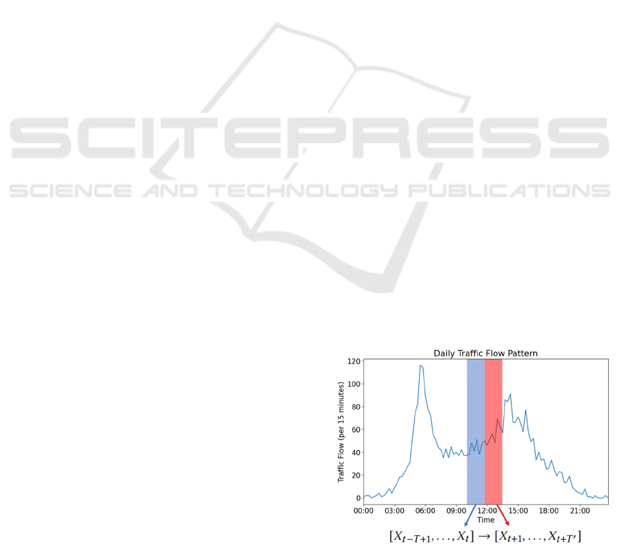
network for each interval. In this paper, we focus our
experiment on traffic flow as the traffic state to be
predicted as illustrated in Figure 1.
Figure 1: Illustration of traffic flow prediction problems.
Spatial Performance Indicators to Evaluate Spatiotemporal Traffic Prediction
157

3 SPATIAL PERFORMANCE
INDICATORS
In this paper, we explore three different metrics from
the domain of GIS called Global Moran’s I, Geary’s
C, and Getis-Ord General G. These metrics will
function as spatial KPIs of traffic prediction that
complements the standard KPI to assist stakeholders
in making more informed decisions. The standard
KPI evaluates traffic prediction on a global scale, so
the aims of spatial KPIs is to evaluate traffic
prediction methods in the spatial aspects.
The selected spatial KPIs are simple scalar
metrics that help evaluate the spatial association of
each node performance in the traffic network and
show the distribution of the prediction errors. Insights
from spatial association unveil hidden patterns and
interdependencies among different spatial locations
and contribute to a better understanding of how the
traffic prediction method is affected by spatial
dependencies. The distribution of the prediction
errors is important information for applications such
as traffic signal control where the prediction
performance of each individual node is more
important than the average performance.
3.1 Global Moran’s I
Global Moran’s I (Moran, 1950) is a global measure
of spatial autocorrelation that tests for the relation
between feature values on each location and the
spatial proximity based on covariance. The metric
will evaluate whether the feature values are correlated
with the same feature values across spatial distances,
either positively or negatively. Global Moran’s I is
calculated using the equation (1):
=

∑(


−
̅
)





∑∑

,
(


−̅
)


(

−̅)


∑∑

,





(1)
where  is the number of features, 

is the feature
values in location , ̅ is the average value of all
features in the network, and 
,
is the element of
spatial weights matrix (adjacency matrix of a graph
network). The ranges of Global Moran’s I are
between +1 and -1 with +1 indicating positive spatial
autocorrelation, 0 indicating a random spatial pattern
with no significant spatial autocorrelation, and -1
indicating negative spatial autocorrelation.
Global Moran’s I is an inferential statistic where
the results are explained in the context of the null
hypothesis. The null hypothesis of Global Moran’s I
is whether the spatial distribution of node values
results from random spatial processes. The 

-score is
defined as:


=
−E[]

V[]
(2)
E
[

]
=−1/(−1)
(3)
V
[

]
=E
[


]
−E
[

]

(4)
When the -value (calculated from 

-score) of
Global Moran’s I (denoted as 

-value) is statistically
significant, we can reject the null hypothesis. In this
case, the positive 

-score indicates the existence of
positive spatial autocorrelation in the networks and
vice versa.
3.2 Geary’s C
Geary’s C (Geary, 1954), similar to Global Moran’s
I, is a global measure of spatial autocorrelation. The
difference between Geary’s C and Global Moran’s I
is Geary’s C describe spatial autocorrelation based on
the squared differences between the location of
features while Global Moran’s I is based on
covariance. Geary’s C is defined as
=
−1
∑(


−
̅
)




∑∑

,


−







2
∑∑

,





(5)
where  is the number of features, 

is the feature
values in location , and 
,
is the element of spatial
weights matrix (adjacency matrix of a graph
network). The ranges of Geary’s C value start from 0
to a positive number with a value between 0 to 1
indicating positive spatial autocorrelation (with a
value approaching 0 has stronger correlation), no
spatial autocorrelation if the value is 1, and value
above 1 indicates negative autocorrelation.
3.3 Getis-Ord General G
Getis-Ord General G (Getis & Ord, 1992) is an
inferential statistic with the null hypothesis stating
that there is no spatial clustering of feature values.
The Getis-Ord General G statistic of overall spatial
clustering is given as:
=
∑∑

,








∑∑








,∀

≠
(6)
where  is the number of features, 

is the feature
values in location , and 
,
is the element of spatial
VEHITS 2024 - 10th International Conference on Vehicle Technology and Intelligent Transport Systems
158

weights matrix (adjacency matrix of a graph
network). Assuming that the adjacency matrix cell
value is between 0 and 1, the range of Getis-Ord
General G will be between 0 and 1 too. The 

-score
is defined as:


=
−E[]

V[]
(7)

[

]
=
∑∑

,




( −1)
,∀

≠
(8)

[

]
=
[


]
−
[

]

(9)
When the -value (calculated from 

-score) of
Getis-Ord General G (denoted as 

-value) is
statistically significant, we can reject the null
hypothesis. In this case, positive 

-score indicates
the high values nodes in the networks is more
spatially clustered while negative 

-score indicates
the low values nodes in the networks is more spatially
clustered.
4 EXPERIMENTS
4.1 PeMSD8 Dataset
In these experiments, traffic flow predictions are
conducted on the PeMSD8 dataset which is a
highway traffic dataset from California. The PeMSD8
dataset is a subset of one of the most popular traffic
datasets, PeMS dataset, that includes both traffic flow
data and the graph adjacency matrix of the freeway
networks. The PeMSD8 dataset is specifically chosen
because it has the least number of nodes which should
have more homogenous spatial pattern compared to
larger traffic networks.
The dataset are measured by the Caltrans
Performance Measurement System (PeMS) (Chen et
al., 2001) in real-time every 30 seconds and
aggregated into 5-minute interval time-series data.
The PeMSD8 dataset are measured from the traffic
data in San Bernardino from July to August 2016,
which contains 1979 detectors on 8 roads. Some
redundant detectors are removed to ensure the
minimum distance between each detector is longer
than 3.5 miles and the resulting dataset contains 170
detectors (Guo et al., 2019).
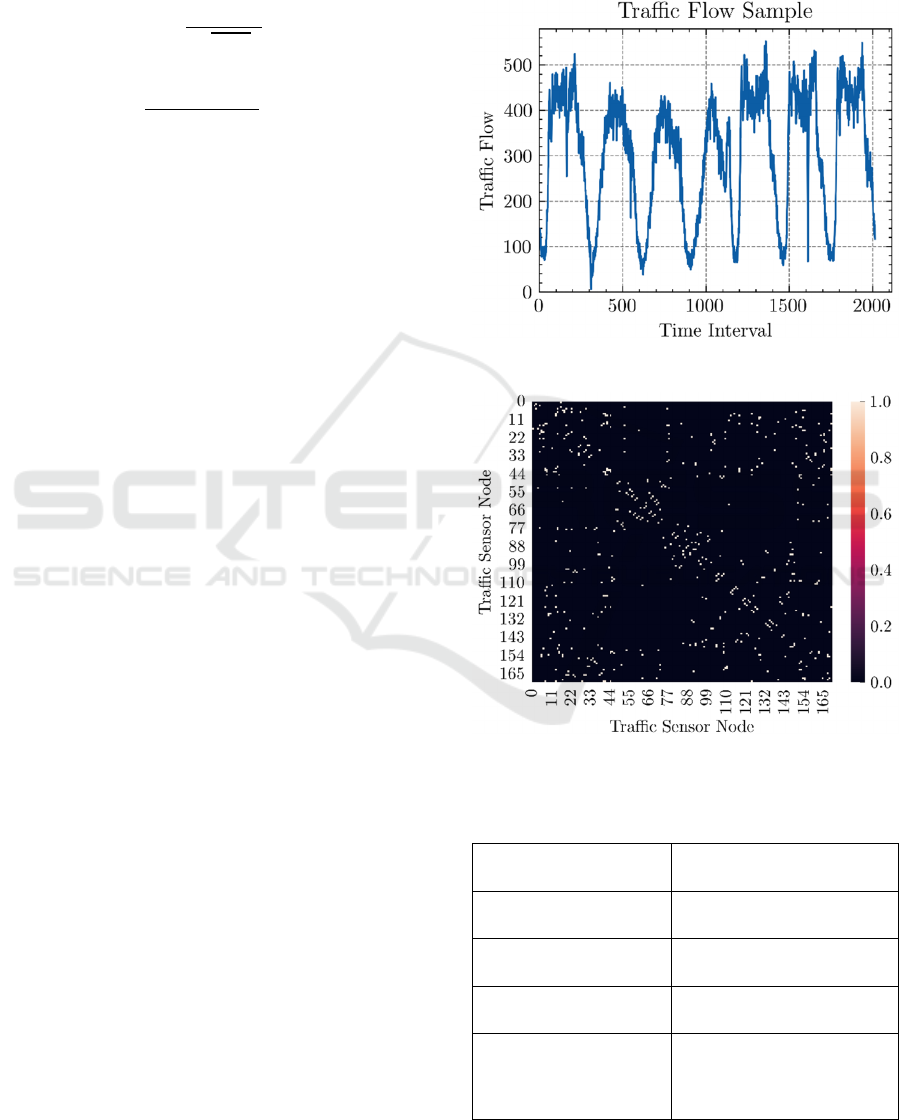
The dataset contains three types of traffic states:
(1) traffic flow (per 5 minutes), (2) traffic speed, and
(3) occupancy, but for our experiments we only use
the traffic flow data as shown in Figure 2. The dataset
contains an adjacency matrix of the traffic sensor
network, enabling graph-based traffic flow prediction
methods that require a predefined graph in the form
of an adjacency matrix as the spatial contexts and
illustrated in Figure 3. The information regarding the
PeMSD8 dataset is summarized in Table 1.
Figure 2: Traffic flow sample from the PeMSD8 dataset.
Figure 3: Adjacency matrix of the PeMSD8 dataset. The
entry , represents an edge from node  to node .
Table 1: Summary of the PeMSD8 dataset.
Number of Nodes 170
Dataset Length 17,856
Dataset Interval 5 minutes
Time Range July 2016 – August 2016
Data Types
Traffic flow, traffic
speed, occupancy, and
adjacency matrix
Spatial Performance Indicators to Evaluate Spatiotemporal Traffic Prediction
159

4.2 Experiment Scenarios
In this paper, the results of traffic flow predictions
will be evaluated with Global Moran’s I, Geary’s C,
and Getis-Ord General G. The experiments are based
on the results of traffic flow predictions of the
PeMSD8 dataset with STSGCN (Song et al., 2020) as
the spatiotemporal predictions method and evaluated
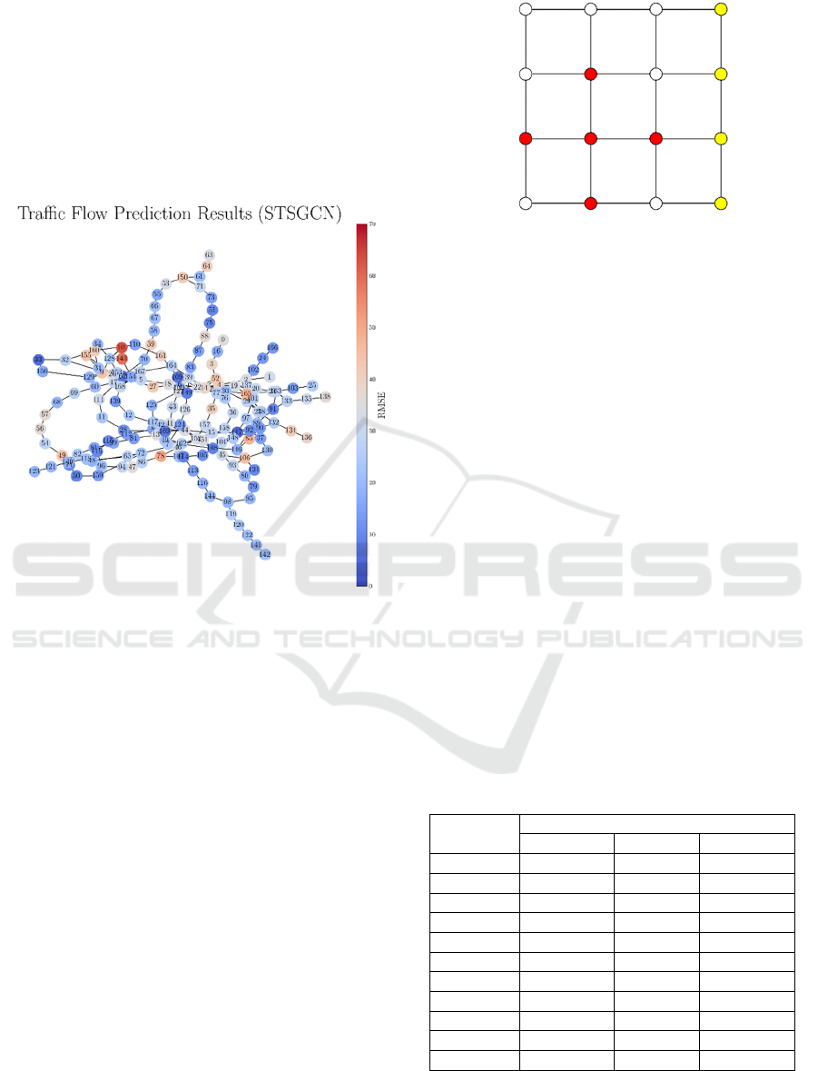
using RMSE on each node as shown in Figure 4.
Figure 4: The results of traffic flow prediction of the
PeMSD8 dataset with STSGCN (Song et al., 2020). The
graph network is automatically generated based on the
adjacency matrix and the colour on each node represents the
RMSE of each node.
To evaluate each spatial KPI for different case
studies, we generate the following scenarios from the
original results as follows:
• Original scenario.
• Two types of clusters (star and line clusters
as illustrated in Figure 5) of high node
values, low node values, and a mix of both
high and low node values.
• Random distribution of high-value nodes.
• Adjust the means of the RMSE results.
• Adjust the variance of the RMSE results.
The aim of the spatial KPIs investigated in this
paper is to capture the spatial association inside the
traffic network and the distribution of the traffic
prediction errors that can’t be evaluated with the
current standard KPI. The scenarios that we created
are aimed at learning what spatial KPIs can capture
and whether the objectives of spatial KPIs could be
fulfilled.
Figure 5: Illustration of different configurations of clusters
in this experiment. Red nodes illustrate star configuration
and yellow nodes illustrate line configuration.
The clustering scenarios reflect the heterogeneity
in the traffic network. In the highway traffic
networks, the heterogeneity arises from factors like
congestion points (for example on-ramps, off-ramps,
and toll booths) and varied land use patterns that
generate spatial clusters of different traffic flow
levels. The urban traffic networks with their different
road hierarchies and intersection dynamics will result
in more complex and heterogeneous networks. This
heterogenous characteristics will be reflected in the
traffic prediction errors distribution but this
information vanishes when the standard KPI averages
prediction errors over the entire traffic network.
For the clustering scenarios, 20 nodes in the traffic
network with the highest or lowest values are
swapped with other nodes to create clusters of nodes
based on the type of clusters. Each clustering scenario
will have an identical average RMSE which is
indistinguishable if the traffic prediction is evaluated
by the standard KPI. Different cluster scenarios and
the number of nodes on each cluster are summarized
in Table 2.
Table 2: Summary of clustering scenarios.
Scenario
Number of Nodes per Cluster
Cluster 1 Cluster 2 Cluster 3
Star HH 10 10 -
Star HL 10 10 -
Star LL 10 10 -
Star H 20 - -
Star L 20 - -
Line HHH 7 8 5
Line HLH 7 8 5
Line LHL 7 8 5
Line LLL 7 8 5
Line HH 14 6 -
Line LL 14 6 -
We consider two types of clusters: high node
values cluster or hotspot and low node values cluster
VEHITS 2024 - 10th International Conference on Vehicle Technology and Intelligent Transport Systems
160

or coldspot denoted as “H” and “L”, respectively. The
distinction is made to evaluate the effects of both
types of clusters and investigate what happens if both
types of clusters exist in the traffic networks. For
example, the “Star HH” scenario point to the graph
network modified to include two high node value
clusters with star configuration and the “Line HLH”
point to the graph network modified to include two
high node value clusters and one low node value
cluster with line configuration.
The scenario of high-value nodes with random
distribution is created to simulate random outliers
happening in the traffic network, similar to salt-and-
pepper noise in digital images. The aim of this
scenario is to evaluate whether spatial KPIs can
differentiate between outlier scattered across the
network and spatially clustered hotspots or coldspots.
The evaluation of spatial KPIs for this scenario
should show significant differences with clustering
scenarios which demonstrate that this scenario has no
spatial association between each outlier nodes.
We also investigate the effects of modifying the
mean and standard deviation of the RMSE of each
node. The aim of modifying the mean of the
prediction errors is to evaluate the sensitivity of
spatial KPIs against different levels of average
prediction errors. The average prediction errors
should be evaluated based on the standard KPI such
as RMSE and shouldn’t affect spatial KPIs. For the
standard deviation modification, the aim is to
evaluate the sensitivity of spatial KPIs against
different standard deviations levels. The change in
both mean and standard deviations occurs when the
data is normalized, and the scenario is to demonstrate
whether such alteration affects spatial KPIs.
5 RESULTS
In these experiments, we will evaluate all different
scenarios with Global Moran’s I, Geary’s C, and
Getis-Ord General G as spatial KPIs. Table 3, Table
4, and Table 5 show Geary’s C, Global Moran’s I, and
Getis Ord General G of all scenarios, respectively.
The confidence level of 90% is chosen for both
Global Moran’s I and Getis-Ord General G so the null
hypothesis can be rejected if the 

-value or 

-value
is under 0.1.
The original scenario which is the results of traffic
flow prediction of the PeMSD8 dataset with
STSGCN (Song et al., 2020) has =0.8260 and
=0.1690 indicating a slight positive spatial
autocorrelation. Both 

-value and 

-value are
under 0.1 with positive 

-score and positive 

-score
indicating the positive spatial autocorrelation and
showing the existence of hotspot. Note that the result
is close to the value of no significant spatial
autocorrelation of =1 and =0 where the graph
network mostly has random spatial distribution with
hotspots as shown in Figure 4.
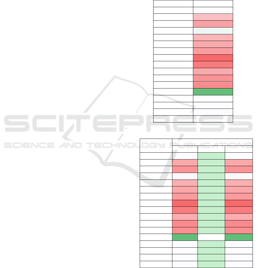
Table 3: Summary of Geary’s C of all scenarios.
Scenario Geary’s C
Original
0.8260
Star HH
0.6928
Star HL
0.6311
Star LL
0.8347
Star H
0.6710
Star L
0.6460
Line HHH
0.6183
Line HLH
0.5045
Line LHL
0.5469
Line LLL
0.6469
Line HH
0.5983
Line LL
0.5799
Random
0.9276
+0.1 mean
0.8260
-0.1 mean
0.8260
+0.1 stdev
0.8260
-0.1 stdev
0.8260
Table 4: Summary of Global Moran’s I of all scenarios.
Scenario
Global Moran's I
I


-value 

-score
Original
0.1690 0.0086 2.6286
Star HH
0.3522 0.0000 5.3797
Star HL
0.3989 0.0000 6.0811
Star LL
0.1801 0.0052 2.7943
Star H
0.3376 0.0000 5.1605
Star L
0.3568 0.0000 5.4500
Line HHH
0.3818 0.0000 5.8253
Line HLH
0.4915 0.0000 7.4726
Line LHL
0.4458 0.0000 6.7858
Line LLL
0.3447 0.0000 5.2672
Line HH
0.4205 0.0000 6.4058
Line LL
0.4117 0.0000 6.2742
Random
0.0692 0.2590 1.1287
+0.1 mean
0.1690 0.0086 2.6286
-0.1 mean
0.1690 0.0086 2.6286
+0.1 stdev
0.1690 0.0086 2.6286
-0.1 stdev
0.1690 0.0086 2.6286
In the random scenario, we shuffle the value of all
nodes randomly and as expected, the results show that
 is close to one and  is close to zero indicating a
random spatial pattern with no significant spatial
Spatial Performance Indicators to Evaluate Spatiotemporal Traffic Prediction
161

autocorrelation. Both 

and 

of the random
scenario are above 0.1 so the null hypothesis can’t be
rejected, indicating a spatial distribution that comes
from random spatial processes. These results show
the capability of spatial KPIs to differentiate between
random distribution of outliers with spatially
clustered hotspots or coldspots.
Table 5: Summary of Getis-Ord General G of all scenarios.
Scenario
Getis-Ord General G
G 

-value 

-score
Original
0.0205 0.0273 1.9220
Star HH
0.0250 0.0000 7.9946
Star HL
0.0219 0.0001 3.8260
Star LL
0.0183 0.1483 -1.0438
Star H
0.0235 0.0000 6.0218
Star L
0.0200 0.1003 1.2797
Line HHH
0.0194 0.3239 0.4567
Line HLH
0.0213 0.0015 2.9586
Line LHL
0.0214 0.0007 3.1764
Line LLL
0.0222 0.0000 4.2612
Line HH
0.0199 0.1201 1.1745
Line LL
0.0219 0.0001 3.8683
Random
0.0198 0.1573 1.0056
+0.1 mean
0.0200 0.0297 1.8845
-0.1 mean
0.0200 0.0247 1.9655
+0.1 stdev
0.0207 0.0250 1.9601
-0.1 stdev
0.0203 0.0301 1.8795
Table 3 shows the results of the evaluation using
Geary’s C for all scenarios. All clustering scenarios
except Star LL show lower  compared to the
original scenario indicating the increases in spatial
autocorrelation because of the clustering. Line
clusters in general have lower  compared to star
clusters which indicates higher sensitivity of Geary’s
C towards line clusters. In both cluster categories, the
lowest  is in the mixed value clusters (Line HLH
and Star HL). In the mixed value clusters, we swap in
a total of 20 nodes from both highest node values and
lowest node values to create clusters of high node
values and low node values so the total of squared
difference 

−



will be higher compared to
other scenarios resulting in lower . In both cluster
categories, larger but fewer clusters have lower 
suggesting higher spatial autocorrelation compared to
smaller but more clusters.
Table 4 shows the results of the evaluation using
Global Moran’s I for all scenarios. All clustering
scenarios are showing larger  than the original
scenario indicating positive spatial autocorrelation
from the clustering. With a sufficiently large number
of nodes, we can test the statistical significance of the
Global Moran’s I. Out of all scenarios, the 

-value
that is not significant is only on the random scenario
which indicates the rejection of the null hypothesis
with all scenarios having positive 

-score that shows
positive spatial autocorrelation. Similar to Geary’s C,
line clusters show higher  and 

-score compared to
star clusters indicating better sensitivity for line
clusters. The mixed clusters for both clustering
categories also have the largest  and 

-score
because of higher covariance (

−̅)(

−̅) .
Larger but fewer clusters also have higher 
indicating higher spatial autocorrelation compared to
smaller but more clusters.
In general, both Global Moran’s I and Geary’s C
show similar trends for all scenarios as both KPIs
measure global measures of spatial autocorrelation.
The level of spatial autocorrelation helps gauge how
much the spatial context influences the prediction
errors. Strong spatial autocorrelation suggests that
incorporating more spatial information into the
prediction model could be beneficial and vice versa.
Based on equation (1) and equation (5), the difference
between the two is Global Moran’s I use covariance
(

−̅)(

−̅) while Geary’s C use squared
differences 

−



. The choice between Global
Moran’s I and Geary’s C are dependent on the
purpose of the KPI. Global Moran’s I have values
ranges between -1 and 1 which makes it more
interpretable and intuitive for both positive spatial
autocorrelation and negative spatial autocorrelation.
Squared differences in Geary’s C make the KPI more
sensitive to spatial outliers and better suited for
detecting dispersion or negative spatial
autocorrelation.
Table 5 shows the results of the evaluation using
Getis-Ord General G for all scenarios. For the Getis-
Ord General G, we will focus the results by
evaluating the 

-value and 

-score as the G value’s
difference between all scenarios are very close and
linear with the 

-value and 

-score.
In the star cluster scenarios, scenarios that include
hotspots such as Star HH, Star HL, and Star H show
an extremely low 

-value with a higher 

-score
compared to the original scenario. This result
indicates that the Getis-Ord General G is sensitive to
star clusters. Star HH have a higher 

-value
compared to Star H showing that the Getis-Ord
General G is more sensitive to more clusters with
fewer nodes compared to least clusters with more
nodes. The results for both Star LL and Star L are
interesting as both scenarios have 

-value larger
than 0.1 and the null hypothesis can’t be rejected. The
original scenario results show the existence of a
VEHITS 2024 - 10th International Conference on Vehicle Technology and Intelligent Transport Systems
162

hotspot as shown in Figure 4, so we suspect that the
coldspots created in these scenarios cancel each other
out with the existing hotspots resulting in larger 

-
value and lower 

-score.
In the line cluster scenarios, scenarios that include
coldspot have tendencies to have lower 

-value and
higher 

-score which is the opposite of the star
cluster scenarios. Two hotspot scenarios, Line HH
and Line HHH, have 

-value larger than 0.1 and the
null hypothesis can’t be rejected. These findings
suggest that the generated line cluster has the opposite
effects of the star cluster and the Getis-Ord General
G usage for detecting clusters is limited to the star
cluster. The existence of a line cluster might
overshadow the Getis-Ord General G's ability to
detect star clusters, similar to how the hotspot and
coldspot in star clusters cancel each other out.
In general, the Getis-Ord General G allow us to
identify the existence of hotspots and coldspots of the
prediction errors in the network. The KPI also show
whether the distribution of the traffic prediction errors
is spatially clustered. The insights help in pinpointing
specific areas where the prediction method performs
exceptionally well or poorly and will be valuable for
targeted improvements or interventions. It should be
highlighted that the existence of hotspots and
coldspots will cancel each other out. The existence of
both star clusters and line clusters also has the same
effects and must be acknowledged.
Other than the clustering scenarios, we also create
scenarios where the mean of the node values is
modified by adding and subtracting 10% from the
node values without changing the standard deviation.
In other scenarios, we also modify the standard
deviation by ±10% without changing the mean. The
results from both scenarios show no change in both
Geary’s C and Global Moran’s I that indicate no
change in spatial autocorrelation by modifying the
mean and standard deviation. These results indicate
that spatial KPIs are insensitive to different levels of
mean and standard deviation of the prediction errors.
The spatial KPIs are affected only by the spatial
autocorrelation even if traffic prediction methods
with significance prediction error differences are
compared. As for Getis-Ord General G, the value
slightly changes with a higher mean or lower standard
deviation increasing the 

-value which indicates a
lower confidence level of the cluster existences.
6 CONCLUSIONS
In this paper, we address the lack of traffic prediction
KPI outside the standard average accuracy KPI,
especially for traffic prediction problems. Three
spatial metrics commonly used in the GIS domain:
Global Moran’s I, Geary’s C, and Getis-Ord General
G are proposed to evaluate the performance of traffic
flow predictions on the PeMSD8 dataset, a freeway
traffic dataset, using STSGCN (Song et al., 2020).
We focus on the spatiotemporal methods and assume
the knowledge of the structure of the traffic network
in the form of a graph adjacency matrix. Several
synthetic scenarios are created from the original
results to show insights that can be captured from
each spatial KPI.
Our experiments show that spatial KPIs provide
valuable insights that can’t be captured from the
standard KPI such as MAE, RMSE, and MAPE. It
allows stakeholders to learn not only the average
performance but also how they are spatially related.
Geary’s C and Global Moran’s I effectively identify
spatial autocorrelation induced by clustering
scenarios. Both methods show higher sensitivity
towards line clusters compared to star clusters. The
results also suggest that larger but fewer clusters have
higher spatial autocorrelation compared to smaller
but more clusters.
The knowledge of the spatial autocorrelation in
the traffic network provides information on how the
spatial context affects the prediction performance.
Higher spatial autocorrelation suggests utilizing more
spatial contexts in traffic prediction will be helpful
and help stakeholders choose the appropriate
prediction technique. The selection between Global
Moran’s I and Geary’s C hinges on the intended
purpose of the KPI. Global Moran’s I offer
intuitiveness for both spatial and negative spatial
autocorrelation while Geary’s C exhibits heightened
sensitivity to spatial outliers that is useful for
detecting dispersion patterns.
Getis-Ord General G can help identify the
existence of clustering in the network, especially star
clusters. Our findings indicate that Getis-Ord General
G can identify the existence of hotspots and coldspots
of the prediction errors in the traffic network. This
information helps stakeholders locate areas in the
traffic network with good or bad prediction errors for
targeted improvements. It should be noted that the
existence of hotspots and coldspots in the network
will cancel each other out. A similar effect is also
observed in the presence of both star clusters and line
clusters.
Future work can investigate traffic prediction of
other traffic states such as speed and travel time.
Experiments in this paper have been limited to
freeway traffic settings, so the validation of the
proposed KPIs in the arterial or urban traffic network
Spatial Performance Indicators to Evaluate Spatiotemporal Traffic Prediction
163

settings is essential to extend the usage of spatial KPIs
to a wider range of applications. Furthermore,
exploring other temporal KPIs and spatial KPIs is
also important to gain more insights in traffic
prediction evaluation. At last, the integration of
spatial KPIs with temporal KPIs is a critical step
towards a better evaluation of traffic prediction
models.
REFERENCES
Adepeju, M., Rosser, G., & Cheng, T. (2016). Novel
evaluation metrics for sparse spatio-temporal point
process hotspot predictions—A crime case study.
International Journal of Geographical Information
Science, 30(11), 2133–2154. https://doi.org/10.1080/
13658816.2016.1159684
Chen, C., Petty, K., Skabardonis, A., Varaiya, P., & Jia, Z.
(2001). Freeway Performance Measurement System:
Mining Loop Detector Data. Transportation Research
Record: Journal of the Transportation Research Board,
1748(1), 96–102. https://doi.org/10.3141/1748-12
Dietel, J. E. (2003). Recordkeeping integrity: Assessing
records’ content after Enron. Information Management
Journal, 37(3), 43–51. ProQuest Central; Social Science
Premium Collection.
Fisher, C. W., Lauria, E. J. M., & Matheus, C. C. (2009).
An Accuracy Metric: Percentages, Randomness, and
Probabilities. Journal of Data and Information Quality,
1(3), 16:1-16:21. https://doi.org/10.1145/1659225.165
9229
Geary, R. C. (1954). The Contiguity Ratio and Statistical
Mapping. The Incorporated Statistician, 5(3), 115–146.
https://doi.org/10.2307/2986645
Getis, A., & Ord, J. K. (1992). The Analysis of Spatial
Association by Use of Distance Statistics. Geographical
Analysis, 24(3), 189–206. https://doi.org/10.1111/
j.1538-4632.1992.tb00261.x
Guo, S., Lin, Y., Feng, N., Song, C., & Wan, H. (2019).
Attention Based Spatial-Temporal Graph
Convolutional Networks for Traffic Flow Forecasting.
Proceedings of the AAAI Conference on Artificial
Intelligence, 33(01), Article 01. https://doi.org/10.16
09/aaai.v33i01.3301922
Korecki, M., Dailisan, D., & Helbing, D. (2023). How Well
Do Reinforcement Learning Approaches Cope With
Disruptions? The Case of Traffic Signal Control. IEEE
Access, 11, 36504–36515. https://doi.org/10.1109/
ACCESS.2023.3266644
Li, L., Tsui, K.-L., & Zhao, Y. (2022). An Overview and
General Framework for Spatiotemporal Modeling and
Applications in Transportation and Public Health. In A.
Steland & K.-L. Tsui (Eds.), Artificial Intelligence, Big
Data and Data Science in Statistics: Challenges and
Solutions in Environmetrics, the Natural Sciences and
Technology (pp. 195–226). Springer International
Publishing. https://doi.org/10.1007/978-3-031-07155-
3_8
Mehdiyev, N., Enke, D., Fettke, P., & Loos, P. (2016).
Evaluating Forecasting Methods by Considering
Different Accuracy Measures. Procedia Computer
Science, 95, 264–271. https://doi.org/10.1016/j.proc
s.2016.09.332
Moran, P. A. P. (1950). Notes on Continuous Stochastic
Phenomena. Biometrika, 37(1/2), 17–23. https://
doi.org/10.2307/2332142
Song, C., Lin, Y., Guo, S., & Wan, H. (2020). Spatial-
Temporal Synchronous Graph Convolutional
Networks: A New Framework for Spatial-Temporal
Network Data Forecasting. Proceedings of the AAAI
Conference on Artificial Intelligence, 34(01), Article
01. https://doi.org/10.1609/aaai.v34i01.5438
Tascikaraoglu, A. (2018). Evaluation of spatio-temporal
forecasting methods in various smart city applications.
Renewable and Sustainable Energy Reviews, 82, 424–
435. https://doi.org/10.1016/j.rser.2017.09.078
Wu, D., Gao, L., Chinazzi, M., Xiong, X., Vespignani, A.,
Ma, Y.-A., & Yu, R. (2021). Quantifying Uncertainty
in Deep Spatiotemporal Forecasting. Proceedings of the
27th ACM SIGKDD Conference on Knowledge
Discovery & Data Mining, 1841–1851. https://doi.org/
10.1145/3447548.3467325
VEHITS 2024 - 10th International Conference on Vehicle Technology and Intelligent Transport Systems
164