
Interpolation-Based Learning for Bounded Model Checking
Anissa Kheireddine
1
, Etienne Renault
2
and Souheib Baarir
1,3
1
LIP6, Sorbonne Universit
´
e, Paris, France
2
SiPearl, Maisons-Laffitte, France
3
Universit
´
e Paris-Nanterre, Nanterre, France
Keywords:
Bounded Model Checking, SAT, Craig Interpolation, Parallelism, Pre-Processing.
Abstract:
In this paper, we propose an interpolation-based learning approach to enhance the effectiveness of solving the
bounded model checking problem. Our method involves breaking down the formula into partitions, where
these partitions interact through a reconciliation scheme leveraging the power of the interpolation theorem to
derive relevant information. Our approach can seamlessly serve two primary purposes: (1) as a preprocessing
engine in sequential contexts or (2) as part of a parallel framework within a portfolio of CDCL solvers.
1 INTRODUCTION
Model checking (Clarke et al., 2009) is an automated
procedure that establishes the correctness of hardware
and software systems. In contrast to testing, it is a
complete and exhaustive method. Model checking is
therefore an essential industrial tool for eliminating
bugs and increasing confidence in hardware designs
and software products. Usually, the studied program
(model) is expressed in a formal language whereas
the property to be checked is expressed as a formula
in some temporal logic (e.g., LTL (Rozier, 2011),
CTL (Clarke and Emerson, 1982)). A property is said
to be verified if no execution of the model can invali-
date it, otherwise, it is violated. To achieve this veri-
fication a (full) traversal of the state-space, represent-
ing the behaviors of the model, is required. Two ap-
proaches have been considered: explicit model check-
ing (Holzmann, 2018) and symbolic model check-
ing (Clarke et al., 1996). In symbolic model check-
ing, states of the studied system are represented im-
plicitly using Boolean functions. From that, mod-
ern satisfiability (SAT) solvers have since become
one of the core technology of many model checkers,
greatly improving capacity when compared to Binary
Decision Diagrams-based model checkers (Biere and
Kr
¨
oning, 2018). In particular, SAT procedures find
extensive application in the bounded version of model
checking, specifically for verifying LTL specifica-
tions. Bounded model checking (BMC) (Biere et al.,
2003) refers to a model checking approach where
the verification of the property is performed using a
bounded traversal, i.e., a traversal of symbolic repre-
sentation of the state-space that is bounded by some
integer k. Such an approach does not require storing
state-space and hence, is found to be more scalable
and useful (Zarpas, 2004). Within this context, nu-
merous optimizations have been developed to guide
SAT procedures towards promising search spaces, ul-
timately reducing the solving times. One particularly
noteworthy optimization involves the generation and
utilization of high-quality (learnt) clauses from Con-
flict Driven Clause Learning-like SAT solvers (Silva
and Sakallah, 1997; Moskewicz et al., 2001). The pri-
mary emphasis of this paper is to enhance the learn-
ing mechanisms within the realm of SAT-based BMC
problems. We explore a clause learning framework
that leverages Craig interpolation (Dreben, 1959).
Firstly, we introduce a novel decomposition method
tailored specifically for BMC problem-solving that
decomposes the SAT formula into independent sub-
parts. Secondly, we harness the interpolation mecha-
nism as a means to generate learnt clauses. To do so,
we took inspiration from the work in (Hamadi et al.,
2011). These learnt clauses are then used in two dis-
tinct dimensions:
• Interpolants as a Preprocessing Engine: within
a sequential context, our approach harnesses the
introduction of interpolants before the solving.
This enhances the efficiency of the SAT solving
process by introducing valuable clauses derived
from interpolation.
• Interpolants in a Parallel Environment: To fur-
ther leverage the wealth of information provided
Kheireddine, A., Renault, E. and Baarir, S.
Interpolation-Based Learning for Bounded Model Checking.
DOI: 10.5220/0012703500003687
Paper published under CC license (CC BY-NC-ND 4.0)
In Proceedings of the 19th International Conference on Evaluation of Novel Approaches to Software Engineering (ENASE 2024), pages 605-614
ISBN: 978-989-758-696-5; ISSN: 2184-4895
Proceedings Copyright © 2024 by SCITEPRESS – Science and Technology Publications, Lda.
605

by interpolants, we extend the application of in-
terpolants into parallel environments by sharing
these interpolants to guide other CDCL solvers
towards promising search spaces. This collabo-
rative approach among solvers improves their col-
lective reasoning capabilities and ultimately leads
to more efficient problem-solving.
The paper structure starts by reviewing important con-
cepts in Section 2 before positioning our work in Sec-
tion 3 to state-of-the-art approaches. Section 4 recalls
the random decomposition of (Hamadi et al., 2011)
and our BMC-based decomposition. Sections 5 and 6
study the effectiveness of interpolation-based learning
on both sequential and parallel settings, respectively.
2 PRELIMINARIES
2.1 SAT Procedures
The satisfiability problem (SAT) is the canonical NP-
complete problem that aims to determine whether
there exists an assignment of values to the Boolean
variables of a propositional formula that makes the
formula true (Cook, 1971). Despite its theoretical
complexity, SAT has evolved into a widely embraced
methodology for tackling challenging problems, par-
ticularly in the realm of formal verification.
Formally, a literal is a Boolean variables or its
negation. A clause c is a finite disjunction of liter-
als. A conjunctive normal form (CNF) propositional
formula F is a finite conjunction of clauses. For a
given F, the set of its variables is noted V . We use
V (c) to denotes the set of variables composing the
clause c. An assignment α of the variables of F is a
function α : V −→ {⊤, ⊥}. α is total (complete) when
all elements of V have an image by α, otherwise it is
partial. For a given formula F and an assignment α,
a clause of F is satisfied when it contains at least one
literal evaluated to true regarding α. F is satisfied by
α iff all clauses of F are satisfied. F is said to be SAT
if such an α exists. It is UNSAT otherwise.
In this work, we are interested in the CDCL al-
gorithm for solving F with significant improvements
that considerably enhance its efficiency. CDCL
incorporates the concept of learning into the DPLL
algorithm (Davis et al., 1962)
1
, making it possible
to learn from conflicts (past errors) in order to avoid
similar decision errors in the future.
1
The overall concept of DPLL has been kept in modern
CDCL algorithms.
2.2 SAT-Based Bounded Model
Checking
The SAT-based BMC approach constructs a proposi-
tional formula that captures the interplay between the
system and the negation of the specification to be ver-
ified, both unrolled up to a given bound, denoted here
by k. When this propositional formula is proven to be
satisfiable (SAT), it implies the presence of a property
violation within a maximum length of k. Conversely,
when the formula is unsatisfiable (UNSAT), it affirms
that the property holds up to length k.
Consider a Kripke structure denoted as M =
⟨S, T, I, AP, L⟩, which represents the system under
study where S is the set of states, T is the transition
relation over the states of S, I ∈ S represents the set of
initial states, AP is a set of atomic propositions, and L
is a labeling function. The negation of the property to
be checked on M is represented by an LTL formula ϕ.
The propositional formula [[M, ϕ]]
k
defines the BMC
problem for ϕ over M w.r.t. k:
[[M, ϕ]]
k
=
Initial states
z}|{
I(s
0
) ∧
k−1
^
i=0
transition relation
z }| {
T (s
i
, s
i+1
)
| {z }
Model
∧
k
^
j=0
[[ϕ]]
j
| {z }
Property
(1)
At time step i, s
i
encompasses truth value assignments
to the set of state variables. The expression [[ϕ]]
k
translates the property into its unrolled from up to k.
2.3 Craig Interpolation
The Craig interpolation theorem (Dreben, 1959) pro-
vides a powerful tool for analyzing the relationship
between two formulas A and B in the context of satis-
fiability. It guarantees the existence of an interpolant
when A ∧ B =⇒ ⊥, allowing us to extract additional
information about the logical structure of A and B.
Given an unsatisfiable conjunction of formulas,
specifically A ∧ B, an interpolant, denoted by I, is a
formula that adheres to the following properties: (i)
A =⇒ I: This implies that if A holds true, then I must
also be true; (ii) B ∧ I =⇒ ⊥: The conjunction of B
and I is unsatisfiable, indicating that there is no as-
signment of variables that simultaneously satisfies B
and I; (iii) I is defined over the common language of
A and B: I is constructed using variables that appear
in both A and B, ensuring that it captures the relevant
information shared by both formulas. The interpolant
I provides an over-approximation of formula A while
still conflicting with formula B. It can be thought of
I as a logical abstraction of A that captures the essen-
tial features needed to demonstrate the conflict with
ENASE 2024 - 19th International Conference on Evaluation of Novel Approaches to Software Engineering
606
B. While the Craig interpolation theorem guarantees
the existence of an interpolant, it does not provide an
algorithm for finding it. However, there are known al-
gorithms for generating interpolants for various log-
ics. One common approach is to derive an interpolant
for A ∧ B from a proof of unsatisfiability of the con-
junction. By analyzing the proof structure, it is possi-
ble to extract the necessary information to construct
the interpolant. In the context of SAT procedures,
McMillan’s interpolation (McMillan, 2003) has been
widely employed. It has been shown to be competi-
tive with SAT solving algorithms and can provide ef-
fective interpolants for model checking problems. To
gain a deeper understanding of McMillan’s interpola-
tion and other interpolation systems, a complete study
can be found in (D’Silva, 2010).
2.4 An Interpolant-Based Decision
Procedure
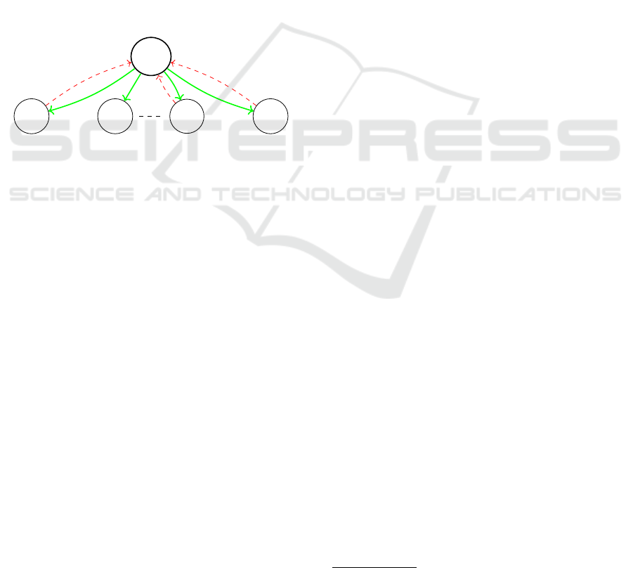
G
ψ
1
UNSAT
ψ
2
SAT
ψ
n−1
UNSAT
ψ
n
UNSAT
α
I
1
α
α
I
n−1
α
I
n
Figure 1: Reconciliation scheme.
The section outlines the framework proposed
in (Hamadi et al., 2011), describing an interpolation-
based decision procedure for SAT formulas. The
main idea is to compute partial solutions for different
parts of the formula at hand and then calculate a
global solution using interpolation mechanisms.
Indeed, they implemented the reconciliation schema
depicted in Figure 1, where partitions of the formula
are reconciled through the variables they share.
Let’s denote by ψ
i
for i = 1, . . . , n, the subfor-
mulas of the studied problem F. These subformulas
are solved by individual SAT solver units. However,
when the partitions happen to share variables (i.e.,
V (ψ
i
) ∩ V (ψ
j
) ̸=
/
0, for some j ̸= i), the resolutions
of the different partitions must be reconciled and syn-
thesized into a feasible global solution. To do so, an-
other solver is added to the schema. Named as the
manager G, it is responsible for reconciling the solu-
tions returned by each partition into a feasible global
solution that satisfies the entire formula F. The recon-
ciliation procedure is built using the following lemma:
Lemma 1. Let F = ψ
1
∧·· · ∧ψ
n
and let α be a partial
solution provided by G that covers the shared vari-
ables, V (G):
V (G) =
n
[
i, j=1,i̸= j
V (ψ
i
) ∩ V (ψ
j
).
If I is an interpolant between ¬ψ
i
and ¬α for any
1 ≤ i ≤ n, then F =⇒ I.
The resulting interpolants I
i
(red arrows in Fig. 1)
from ¬(ψ
i
∧ α) are added into G, effectively remov-
ing the partial solution α (green arrows in Fig. 1) in
future iterations.
Using the above lemma, the authors of (Hamadi et al.,
2011) present a reconciliation algorithm, for solving
SAT problems using any decomposition method. The
algorithm takes as input a CNF formula F and a num-
ber of partitions n.
The entire procedure has been implemented in a
framework called DESAT
2
. It integrates the McMil-
lan interpolation (McMillan, 2003) and the lazy de-
composition that will be detailed in Section 4.1. DE-
SAT uses MINISAT1.14P (E
´
en and S
¨
orensson, 2003)
as a core engine. This older version of MINISAT has
the ability to provide a proof of unsatisfiability.
3 RELATED WORKS
(Hamadi et al., 2011) used an interpolation-based
technique when treating formulas that are too large
to be handled by a single computing unit. To achieve
this, they propose decomposing the formulas into par-
titions that can be solved by individual computing
units. Once each partition is solved, the partial re-
sults are combined using Craig interpolation (Dreben,
1959) to obtain the overall result. However, the pro-
posed approach did not use any structural information
of the problem at hand.
Apart from the usage of interpolation mecha-
nisms in IC3 (Bradley, 2012), PDR (Een et al.,
2011) and some usage in the incremental SAT-based
BMC (Wieringa, 2011; Sery et al., 2012; Cabodi
et al., 2017), to the best of our knowledge, no one
has explored their usage on one single BMC instance.
The most closely work related to ours is (Ca-
bodi et al., 2017). This preliminary research pro-
poses to extract information from an interpolant-
based model-checking engine during the solving pro-
cess (in-processing). They manage to derive an over-
approximation of fixed time frames with the aim
of early detecting invalid variable assignments at a
specific time frame. This initial study can provide
additional insights when integrated with our ongo-
ing work, where pre-processing and in-processing
interpolation procedures are simultaneously applied.
However, it’s worth noting that the effectiveness of
2
https://www.winterstiger.at/christoph/
Interpolation-Based Learning for Bounded Model Checking
607

this approach for various types of specifications is not
known, as their study was exclusively applied to in-
variant properties, while our approach is applied for
any type of LTL property.
In the context of parallel computing, the au-
thors of (Ganai et al., 2006) extended the concept
from (Zhao et al., 2001) to the domain of BMC. This
method involves distributed-SAT solving across a net-
work of workstations using a Master/Client model,
wherein each Client workstation holds an exclusive
partition of the SAT problem. The authors of (Ganai
et al., 2006) optimized the communication within the
context of BMC by introducing a structural partition-
ing approach. This strategy allocates each processor
a distinct set of consecutive BMC time frames. As
a result, when a Client workstation completes unit
propagation on its assigned clauses, it only broadcasts
the newly implied variables to specific Clients. This
allows for effective communication between Clients
and ensures that receiving Clients never need to pro-
cess a message not intended for them. Besides, the
works of (Kheireddine et al., 2023) provide a new
metric to identify relevant learnt clauses based on
the variable origins from BMC problems. The au-
thors propose some heuristics based on this measure
to tune the learnt clause databases of CDCL SAT
solver. They also employ these heuristics to redefine
the clause exchange policy between multiple CDCL
solvers in a parallel context.
4 DECOMPOSITION-BASED
STRATEGIES
To formally explore the idea mentioned in Sec-
tion 2.4, we begin by examining how the formula is
decomposed. We first study the initial decomposition
proposed in (Hamadi et al., 2011), and then we detail
our new splitting method tailored to the BMC prob-
lem.
Throughout this work, we maintain using the DE-
SAT framework (cited in Section 2.4) for all the pre-
sented experiments since the framework DESAT al-
ready has the interpolation algorithms and the rec-
onciliation mechanism in place. The integration of
a modern SAT solver, like CADICAL (Biere et al.,
2021), is in our perspective.
4.1 Lazy Decomposition (LZY-D)
The process of finding sparsely connected partitions
in a formula and eliminating connections to make
the partitions independent is not a straightforward
operation. Hamadi et al. (Hamadi et al., 2011) pro-
pose a computationally-free decomposition (LZY-D),
known as lazy decomposition:
Definition Lazy Decomposition (LZY-D). Let F be
in conjunctive normal form of q clauses, i.e., F =
F
1
∧ · ·· ∧ F
q
. A lazy decomposition of F into n par-
titions is an equivalent set of formulas ψ
1
, . . . , ψ
n
,
where each ψ
i
is equivalent to some conjunction of
clauses from F. In other words, there exist integers
a and b (with a < b ≤ q) such that ψ
i
= F
a
∧ ··· ∧ F
b
.
The lazy decomposition approach (LZY-D) does not
explicitly enforce independence among the partitions.
Instead, it divides the clauses of the problem into a
number of equally sized partitions. The clauses are
ordered as they appear in the input file, and each par-
tition ψ
i
is assigned the clauses numbered from i·⌊
q
n
⌋
to (i + 1) · ⌊
q
n
⌋.
4.2 BMC Decomposition (BMC-D)
Cutting the set of clauses randomly remains a generic
approach which does not require the knowledge of
the problem’s structure. Indeed, consider the spe-
cific structure of a BMC problem, characterized by
a finite state system. As the system operates on dis-
crete states, each state can be represented by a set of
variables and its corresponding constraints in the SAT
formula. It becomes evident that isolating each state
encoding from the SAT formula is a straightforward
task. By leveraging this inherent structure, we can
partition the SAT-based BMC formula into subformu-
las based on the k + 1 states of the system (k steps
+ initial state). This finer decomposition will allow
us to create (relatively) more independent and smaller
subproblems. Moreover, it enables the prediction of
relevant information about the system’s behavior to
easily split potential error paths through the genera-
tion of precise interpolants.
In light of this observation, we propose a
decomposition-based BMC (BMC-D) approach that
takes advantage of the problem’s structure
3
.
From the encoding of BMC problem into proposi-
tional formula 1, the partitioning approach we pro-
pose is based on system states, where each partition
ψ
i
, i = 1 . . . n, is assigned a subset of adjacent states
of equal size t = ⌊
k+1
n
⌋:
ψ
i
=
i·t−2
^
j=(i−1)·t
T (s
j
, s
j+1
) ∧
i·t−1
^
j=(i−1)·t
[[ϕ]]
j
(2)
Each partition encompasses a segment of the transi-
tion unrolling as well as the constraints encoding a
3
Source code are available in: https://github.com/
akheireddine/DECOMP-BMC
ENASE 2024 - 19th International Conference on Evaluation of Novel Approaches to Software Engineering
608
portion of the property ϕ. The partitions on both ends,
ψ
1
and ψ
n
, contain more information than the internal
partitions that follow the above formula 2:
– ψ
1
includes constraints of the initial states
I(s
0
) .
– ψ
n
includes the
remaining last transition constraints .
Example. Consider a partitioning with n = 4 for a
BMC problem that has been unrolled up to bound k =
20 that verifies an invariant property (e.g., G p for any
p ∈ AP). Each partition groups t = ⌊
21
4
⌋ = 5 frames.
V (ψ
1
) contains variables of steps s
0
to s
4
, implying
that:
• constraints assigned to ψ
1
are I(s
0
) ∧T (s
0
, s
1
) ∧
··· ∧ T (s
3
, s
4
) ∧ [[ϕ]]
0
∧ ··· ∧ [[ϕ]]
4
,
• ψ
2
encloses variables of s
5
to s
9
, i.e., T (s
5
, s
6
) ∧
··· ∧ T (s
8
, s
9
) ∧ [[ϕ]]
5
∧ ··· ∧ [[ϕ]]
9
,
• ψ
3
are T (s
10
, s
11
)∧··· ∧ T (s
13
, s
14
)∧[[ϕ]]
10
∧···∧
[[ϕ]]
14
, and,
• ψ
4
with T (s
15
, s
16
) ∧ · · ·∧ T (s
19
, s
20
) ∧[[ϕ]]
15
∧
··· ∧ [[ϕ]]
20
.
Two successive partitions ψ
i
and ψ
i+1
are con-
nected, respectively, through the last and first states
of the partitions. In the example above, partitions ψ
1
and ψ
2
are connected through the transition T (s
4
, s
5
)
where state s
4
is included in the first partition ψ
1
and
s
5
on ψ
2
. Thus, this transition involves variables from
both partitions. Due to the ambiguity of including
these frames in either ψ
i
or ψ
i+1
, it is reasonable
for the partition G to integrate them into its clause
database. This ensures consistent decisions across
different partitions and prevents conflicting decisions
regarding the shared variables.
This last observation leads to a modification of the
reconciliation algorithm, where G is initialized with a
subset of the problem’s clauses corresponding to the
transitions linking the n partitions together. This ini-
tialization also encompasses a segment of the prop-
erty’s constraints. This adaptation proves particularly
relevant for certain types of formulas whose interpre-
tation involves adjacent time steps. For instance, con-
sider the specification ”G X p” for any p ∈ AP. Its
propositional formula encoding implies variables at
time steps i and i + 1, which correspond to states s
i
and s
i+1
of the system’s automaton. This implies that
G incorporates the following constraints of the prob-
lem:
G =
N
^
i=1
T (s
i·t−1
, s
i·t
) ∧
n−1
^
j=1
n
^
j<l
j
[[ϕ]]
l
with N =
(
n if n mod k = 0
n − 1 otherwise
where
j
[[ϕ]]
l
represents the property’s constraints that
entail the j-th and l-th partitions, i.e., a state from ψ
j
is linked to a state in ψ
l
in the property formula.
Hence, G will be in charge of deciding on the follow-
ing shared variables:
V (G) =
n−1
[
i=1
V (ψ
i
) ∩ V (ψ
i+1
)
| {z }
common variables
between two partitions
[
V
G
|{z}
variables composing
G’s clauses
When solving G, the process involves the assign-
ing of values to a subset of the whole formula’s vari-
ables (V (G) ⊂ V (F)). This approach narrows down
the focus to a limited set of variables, thereby decreas-
ing the communication overhead with the partitions.
It’s worth noting that G has a partial view of the prob-
lem, incorporating the transitions between successive
partitions. Each partition can be seen as a represen-
tation of a portion of the paths connecting the initial
state s
0
(contained in ψ
1
) to the final state s
k
(in ψ
n
).
Consequently, the generated partial assignments α are
constructed in a way that aligns the partitions in order
to identify a complete path that violates the property.
Where, in contrast, the manager G of LZY-D starts
with no initial constraints. This decomposition is con-
ducted randomly, distributing constraints encoding a
transition or property constraints at a fixed depth un-
evenly among partitions. The following subsection
will allow a comparison of these two decomposition
methods.
4.3 Comparing LZY-D and BMC-D
Hamadi et al.’s approach was originally designed as
a complete decision procedure for satisfiability prob-
lems. However, it heavily relies on computationally
intensive methods, with interpolation being the pri-
mary one. This characteristic diminishes its practical
feasibility for direct application. Nevertheless, it is
entirely conceivable to adapt and reuse this approach
for other purposes. One potential utility lies in using
it as a pre-processing tool or on a parallel context that
furnishes insights about the problem at hand, thereby
assisting classical SAT solvers in achieving more ef-
ficient resolutions. Hence, the idea we will explore in
this paper is to leverage the interpolants generated by
a (potentially partial) execution of this approach as a
set of auxiliary information that can be incorporated
into the original problem.
Nevertheless, we initiated a preliminary series
of experiments with the intention of comparing
Interpolation-Based Learning for Bounded Model Checking
609

Table 1: Comparison of LZY-D and BMC-D decomp. for different partition sizes n.
part. n 5 10 20 30 40 50
#S P #S P #S P #S P #S P #S P
BMC-D 15 622h 28 586h 44 541h 35 561h 21 604h 49 534h
LZY-D 4 654h 6 649h 5 653h 9 642h 10 638h 9 642h
the aforementioned decomposition approaches when
used as complete solving procedures for BMC prob-
lems. This will shed light on the quality of the inter-
polants generated by each approach.
Benchmark Setup. Our BMC benchmark com-
prises SMV (McMillan, 1993) programs. These pro-
grams, along with their respective LTL properties,
have been sourced from a diverse range of bench-
marks, including the HWMC Competition (2017
and 2020
4
), hardware verification problems (Cimatti
et al., 2002), the BEEM database, and the RERS
Challenge
5
. Additionally, certain LTL properties
have been generated using Spot
6
to ensure that each
category of the Manna & Pnueli hierarchy (Manna
and Pnueli, 1990) is represented. We utilized various
bounds k ranging in {60, 80, ..., 1000}. We excluded
trivial instances that executed in less than 1 second on
MINISAT1.14P (E
´
en and S
¨
orensson, 2003).
Table 1 presents the results of 200 randomly
selected BMC problems from the aforementioned
benchmark (mainly composed of safety and persis-
tence properties). The partition sizes used were n =
5, 10, ..., 50, with a time limit of 6000 seconds. We re-
stricted the evaluation to these partition sizes, aligning
with the choices made in the original paper’s experi-
ments (Hamadi et al., 2011), employing the same in-
terpolation algorithm (McMillan (McMillan, 2003)).
The table highlights the number of solved instances
(#S) and the PAR-2
7
time (P).
We observe that BMC-D outperforms LZY-D
significantly, especially when dealing with larger par-
tition sizes (e.g., n = 50). BMC-D successfully
solves 49 instances, leading to a noteworthy reduc-
tion of 108 hours in PAR-2 time compared to LZY-
D. These results seem to imply that the improvement
is attributed to concentrating the majority of clauses
in partition G, resulting in empty partitions within ψ
i
as n approaches the bound k of the considered prob-
lem. This brings us back to the scenario of a stan-
4
http://fmv.jku.at/hwmcc17/,http://fmv.jku.at/hwmcc20/
5
https://tinyurl.com/29a4jcme
6
https://spot.lre.epita.fr/
7
PAR-k is a measure used in SAT competitions that pe-
nalizes the average run-time, counting each timeout as k
times the running time cutoff
dard (flat) resolution. However, our concrete obser-
vations invalidate this hypothesis, revealing that the
ψ
i
partitions do indeed encompass a fair portion of
the problem’s clauses. On the contrary, the BMC-D
strategy helps to separate independent subspaces pro-
viding better performances than LZY-D strategy.
Due to interpolation computation, neither of the
two approaches managed to surpass the performance
of a classical solver (MINISAT1.14P). This is in
contradiction with the reported results in (Hamadi
et al., 2011). Actually, LZY-D fails to outperform
MINISAT1.14P within a verification benchmark con-
text. One potential explanation is that the benchmark,
as pointed out by the authors, is composed of fully
symmetrical problems, whereas the BMC benchmark
contains relatively fewer symmetries than expected:
the conversion of BMC problems into CNF format
disrupts symmetries, largely due to the introduction
of extra variables during the encoding that break out
the symmetry.
In light of these results, we draw two conclusions:
(1) the clauses produced by the interpolants appear
to provide valuable insights, and (2) the current ap-
proach is hindered by the computational complexity
of interpolation. This prompts the question: how
can we leverage these interpolants in an optimal
solving process? Our suggestions for addressing this
question are discussed in the following two sections.
5 INTERPOLATION-BASED
OFFLINE LEARNING
It is intriguing to thoroughly assess the relevance
and quality of information generated by interpola-
tion when compared to that naturally acquired by a
state-of-the-art SAT solver during its learning pro-
cess. Our intuition suggests that clauses derived from
interpolants could be highly beneficial in aiding a
SAT solver, potentially leading to reduced solving
times.
To validate our intuitions and hypothesis, we con-
ducted an experiment employing LZY-D and BMC-
D as pre-processing steps for a CDCL SAT solver.
The primary objective here was to evaluate the infor-
ENASE 2024 - 19th International Conference on Evaluation of Novel Approaches to Software Engineering
610
Table 2: Impact of interpolants’ clauses on the solving.
part. n 5 10 20 30 40 50
#S P #S P #S P #S P #S P #S P
BMC-D-ITP 111 328h 110 333h 111 329h 111 329h 109 331h 110 329h
LZY-D-ITP 109 335h 107 338h 105 341h 110 327h 107 338h 107 338h
original inst. 107 337h
Table 3: Average rate of interpolants size.
part. n 5 10 20 30 40 50 Avg aug.
BMC-D 1.14 % 1.24 % 1.53 % 1.63 % 1.48 % 1.48 % 1.41 %
LZY-D 4.13 % 2.68 % 2.03 % 1.16 % 0.69 % 0.79 % 1.91 %
mation’s value provided by interpolants in contrast
to the information gathered by a conventional SAT
solver, all within the same time constraints. To be
more specific, each of the two algorithms was run
for a limited time period, with a particular partition
size. The interpolants generated during this period
were converted into clauses and added to the initial
instance. We refer to this process as “offline learn-
ing”. The augmented instance was then solved by a
CDCL-like SAT solver.
In this context, we randomly selected a set of 200
BMC instances from the benchmark setup described
in Section 4.3. Each instance underwent an enrich-
ment process involving the incorporation of interpo-
lation clauses generated through offline learning over
a period of 600 seconds. These instances were solved
by MINISAT1.14P within a timeout of 6000 seconds.
For reference, the original instances (without ad-
ditional clauses) were also solved by MINISAT1.14P
within a timeout of 6600 seconds to accommodate the
additional time required for offline learning.
Table 2 highlights the obtained results. BMC-D-
ITP (resp. LZY-D-ITP) indicates the line where in-
stances are augmented with BMC-D (resp. LZY-D)
interpolants. The line labeled as original inst refers to
the original instances without any additional clauses.
The rest of the reported information are the same as
in Table 1. Both decomposition approaches exhibit
improved solving times and succeed in resolving ad-
ditional instances that could not be tackled without
the offline learning. Notably, BMC-D interpolants
have enhanced the solving. It showcases superior per-
formance with a partition size of n = 5, solving 4 in-
stances more and reducing the PAR-2 time by up to
9 hours compared to solving the original problem.
LZY-D decomposition yields better outcomes with
n = 30, solving 3 instances more in 10 hours shorter
than solving the original instances.
These results confirmed our initial intuition re-
garding the significance of information acquired
through the interpolation process. It becomes evident
that the interpolants obtained from the structural de-
composition method BMC-D prove to be more valu-
able compared to those derived from LZY-D.
Indeed, Table 3 illustrates the average percentage
of the number of additional clauses added to the orig-
inal problems, that were learnt by the LZY-D and
BMC-D strategies during the offline learning phase,
and across various partitioning sizes n. The last col-
umn displays the average percentage increase across
all partition sizes.
..... BMC-D decomposition consistently generates
a stable and equivalent set of clauses across all par-
titioning sizes. The increase in the total number
of clauses remains limited, reaching a maximum of
1.63 % of additional clauses, with an average aug-
mentation of 1.41 %. Regardless of the chosen parti-
tion size, on the contrary, the LZY-D approach tends
to produce a larger number of clauses, including up
to 4.13 % of interpolation clauses with an average
augmentation of 1.91 %. We observe a decrease in
the number of generated interpolants relative to the
partition size. These two trends can be explained as
follows: the decomposition-based BMC strategy al-
lowed us to generate a relatively consistent amount
of information within the 600 seconds time frame.
This consistency arises from two related aspects: (a)
the distribution of shared variables between two par-
titions is homogeneous, with the exception of the first
and last partitions, each containing more or less infor-
mation than the others (ψ
1
contains the initial state
I(s
0
) and ψ
n
the remaining states if any). These
shared variables are designed to connect the parti-
tions, thereby identifying a complete path that vio-
lates the property; (b) The partial assignment α, gen-
erated by G, consistently produces conflicts, i.e., in-
terpolants, regardless of the partition size. For in-
stance, when using a partitioning scheme with n = 5
Interpolation-Based Learning for Bounded Model Checking
611
(resp. n = 50), BMC-D generates an average of 4.40
(resp. 34.06) interpolants per round, where a round
signifies when the manager G has traversed all parti-
tions ψ
i
over the current partial assignment α.
..... In contrast, the random partitioning approach
LZY-D generates fewer interpolants per round, with
an average of 1.81 interpolants for n = 5 and 2.86
for a partition size of n = 50. We observed that the
distribution of shared variables is less homogeneous
between partitions. This non-homogeneity arises be-
cause the partitioning is random, leading to some
partitions sharing many more variables than others.
Thus, due to this randomness in the shared variables,
it becomes challenging to produce many conflicts re-
gardless of the given assignment α. Additionally, the
manager G of the LZY-D approach starts with no
constraints in its database, which can result in the
generation of assignments α that do not differ signif-
icantly. Consequently, it becomes more challenging
for G to find a model α that violates a majority of
the partitions, leading to a reduced number of inter-
polants.
..... Based on these measurements, this analysis
clearly underscores the competitive and efficient na-
ture of a decomposition approach that takes into con-
sideration the structural aspects of the BMC problem,
in contrast to a randomized decomposition strategy.
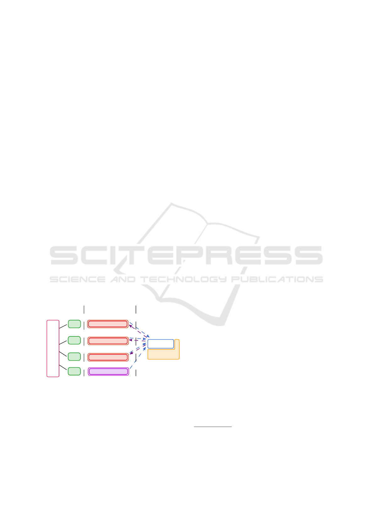
6 INTERPOLATION-BASED
LEARNING IN PARALLEL
SOLVING
Sharing
Parallelization
SW
...
SW
PF
ControlFlow
Sharer
Sequential
Engines
...
CDCL solver
...
CDCL solver
CDCL solver
SW
SW
...
Decomposition-based
Interpolants
solver
Figure 2: Portfolio of solvers with sharing scheme using the
framework PaInleSS.
As demonstrated earlier, interpolation clauses have
a positive impact on the overall resolution time for
BMC problems (refer to Table 2). This finding un-
derscores the potential advantages of integrating our
concept within a parallel computing context. One of
the most effective strategies in parallel SAT solving
is the “portfolio” approach. In essence, a portfolio
consists of a set of sequential SAT solvers that run in
parallel and compete to solve a problem. These core
engine solvers vary in several ways, including the al-
gorithms they employ and their initialization parame-
ters. Moreover, they can exchange information to ex-
pedite problem-solving and avoid repeating the same
mistakes. This aspect forms the basis for the integra-
tion of the approaches discussed thus far. Indeed, we
incorporate our decomposition-based solver, along-
side multiple sequential CDCL engines into a portfo-
lio strategy (via the PAINLESS framework (Le Frioux
et al., 2017)), as illustrated in Figure 2. Three main
components arise when treating parallel SAT solvers:
(i) sequential engines. it can be any CDCL state-
of-the art solver; (ii) parallelization. is represented
by a tree-structure. The internal nodes of the tree rep-
resent parallelization strategies, and leaves are core
engines (SW), and; (iii) sharing. is in charge of re-
ceiving and exporting the set of clauses provided by
the sequential engines during the solving process.
In this integration, the interpolation-derived
clauses are shared among the CDCL solvers. This
aims to enhance the knowledge base of CDCL solvers
and support them throughout the solving process. In
this framework, the decomposition-based solver does
not import information from other solvers; instead, it
exclusively provides its interpolants to them. It func-
tions as a ”black-box”, serving as a specialized clause
generator designed for BMC problems.
For the sake of simplicity, the exchange phase
of the sharing component is to share clauses with a
limited LBD
8
value (Simon and Audemard, 2009).
Specifically, CDCL solvers export learnt clauses iden-
tified by an LBD ≤ 4, a threshold that has been em-
pirically proven to be effective in recent portfolios
9
.
Upon receiving the interpolants from the n parti-
tions, the manager G calculates their corresponding
LBD values and shares only those with LBD ≤ 4, fol-
lowing a similar approach as used for sharing conflict-
ing learnt clauses.
To encourage the solvers to explore diverse search
subspaces, it is essential to introduce some variation
in the solver’s parameters, such as the initial phase of
the variables. By ensuring that each solver runs with
a different initialization phase, they are more likely to
make distinct decisions, leading to exploration of dis-
tinct search subspaces. This diversification approach
will be applied to all the portfolios evaluated in the
subsequent analysis.
8
LBD is a learnt clause quality metric used in almost all
competitive sequential CDCL-like SAT solvers and parallel
sharing strategies.
9
https://satcompetition.github.io/2023/
ENASE 2024 - 19th International Conference on Evaluation of Novel Approaches to Software Engineering
612
Table 4: Performance comparison between Portfolios.
Portfolio part. n SAT UNSAT Total PAR-2
P-BMC-D
5 186 115 301 356h05
50 186 119 305 345h40
P-LZY-D
5 184 113 297 371h09
50 185 113 298 367h20
P-MINISAT - 185 113 298 362h57
Experimental Evaluation
Table 5: Number of solved instances of P-BMC-D for dif-
ferent frame sizes t.
Portfolio
num. steps t
[1 , 7] [8 , 30] [31, 200]
P-LZY-D 0 +12 -1
P-MINISAT +3 +10 -1
The experiments were conducted on the same bench-
mark described in Section 4.3 with 200 additional
BMC instances (400 instances in total). Each in-
stance had a time limit of 6000 seconds for execution.
The portfolio setups comprised 10 threads, and the
solvers used in these portfolio configurations were as
follows: (i) P-MINISAT: The portfolio exclusively
employs the original MINISAT1.14P solver; (ii) P-
BMC-D: One MINISAT1.14P solver was replaced
with a decomposition-based solver using BMC-D de-
composition. (iii) P-LZY-D: Similar to P-BMC-D
portfolio, it incorporates LZY-D instead.
Table 4 presents the results for both smaller (n =
5) and larger (n = 50) partition sizes. The remaining
configurations yielded outcomes similar to those with
n = 5. The table provides information on the number
of solved SAT and UNSAT instances, along with the
total instances and the PAR-2 metrics.
Unsurprisingly, P-BMC-D outperforms the base-
line P-MINISAT by solving 6 more UNSAT instances
and 1 additional SAT instance, all within a remarkable
17 hours reduction in PAR-2 solving time. Further-
more, P-BMC-D exhibits a clear advantage over P-
LZY-D for both partitioning sizes (n = 5, 50), solving
up to 7 more instances and achieving a PAR-2 time re-
duction of up to 21 hours.
Given these results, we sought to examine the re-
lationship between the partitioning size and the un-
rolling depth k of the BMC problem. To do this, we
conducted an analysis in which we categorized the en-
tire benchmark of 400 BMC problems based on the
number of frames within a single partition ψ
i
, noted
t. This categorization was performed for various par-
tition sizes, n = 5, 10, 20, 30, 40, 50.
Table 5 provides an overview of the additional in-
stances solved (+) or lost (-) by P-BMC-D in com-
parison to the P-LZY-D and P-MINISAT portfolios,
indicated in the first and second rows, respectively.
We categorized the BMC problems into three groups
based on the number of frames t contained within
a partition ψ
i
. The first column ([1,7]) includes in-
stances where each partition contains at least one
frame and at most 7 frames (1 ≤ t ≤ 7). The next
column corresponds to instances where t falls within
the range of 8 to 30. Finally, the last column groups
the remaining values of t up to 200. The evaluated
benchmark bounds k varies from 10 to 1000 steps, we
have t =
1000
n
= 200 frames as a limit.
An interesting observation is that clustering a
large number of frames within a single partition (30 <
t ≤ 200) negatively impacts the performance of P-
BMC-D. This is evident from Table 5, where P-
BMC-D failed to solve one instance compared to the
other two portfolios. The most significant improve-
ment is observed when t ∈ [8, 30], where P-BMC-D
solved 10 and 12 additional problems compared to P-
MINISAT and P-LZY-D, respectively. Furthermore,
grouping a small number of frames within a single
partition ([1,7]) only marginally enhances the perfor-
mance of P-BMC-D.
Based on the above analysis, it becomes evi-
dent that utilizing interpolation-based clause learning
through a BMC-based partitioning, which balances
the inclusion of a reasonable number of frames within
each partition (t ∈ [8, 30]), yields the most favorable
outcomes in terms of solving efficiency. This sug-
gests that the granularity of partitioning n and the to-
tal number of frames t within each partition play a key
role in computing relevant interpolants.
7 CONCLUSION
Our objective was to enhance the efficiency of SAT-
based BMC solving by leveraging the interpolation
mechanism to generate learned clauses. Our ongoing
research aims to extend this concept to more recent
solvers, such as CADICAL, which holds the potential
to furnish robust unsatisfiable proofs, consequently
yielding more informative interpolants.
REFERENCES
Biere, A., Cimatti, A., Clarke, E. M., Strichman, O., and
Zhu, Y. (2003). Bounded model checking.
Biere, A., Fleury, M., and Heisinger, M. (2021). CaD-
iCaL, Kissat, Paracooba entering the SAT Competi-
tion 2021. In Balyo, T., Froleyks, N., Heule, M., Iser,
M., J
¨
arvisalo, M., and Suda, M., editors, Proc. of SAT
Interpolation-Based Learning for Bounded Model Checking
613

Competition 2021 – Solver and Benchmark Descrip-
tions, volume B-2021-1 of Department of Computer
Science Report Series B. University of Helsinki.
Biere, A. and Kr
¨
oning, D. (2018). SAT-Based Model Check-
ing, pages 277–303. Springer International Publish-
ing, Cham.
Bradley, A. R. (2012). Understanding IC3. In SAT, volume
7317 of Lecture Notes in Computer Science, pages 1–
14. Springer.
Cabodi, G., Camurati, P., Palena, M., Pasini, P., and Ven-
draminetto, D. (2017). Interpolation-based learning
as a mean to speed-up bounded model checking (short
paper). In Cimatti, A. and Sirjani, M., editors, Soft-
ware Engineering and Formal Methods, pages 382–
387, Cham. Springer International Publishing.
Cimatti, A., Clarke, E., Giunchiglia, E., Giunchiglia, F., Pi-
store, M., Roveri, M., Sebastiani, R., and Tacchella,
A. (2002). NuSMV Version 2: An OpenSource Tool
for Symbolic Model Checking. In CAV 2002, volume
2404 of LNCS, Copenhagen, Denmark. Springer.
Clarke, E., Emerson, E., and Sifakis, J. (2009). Model
checking. Communications of the ACM, 52.
Clarke, E., McMillan, K., Campos, S., and Hartonas-
Garmhausen, V. (1996). Symbolic model checking.
In Alur, R. and Henzinger, T. A., editors, Computer
Aided Verification, pages 419–422, Berlin, Heidel-
berg. Springer Berlin Heidelberg.
Clarke, E. M. and Emerson, E. A. (1982). Design and syn-
thesis of synchronization skeletons using branching
time temporal logic. In Logics of Programs, Berlin,
Heidelberg. Springer Berlin Heidelberg.
Cook, S. A. (1971). The complexity of theorem proving
procedures. In Proceedings of the Third Annual ACM
Symposium, pages 151–158, New York. ACM.
Davis, M., Logemann, G., and Loveland, D. (1962). A ma-
chine program for theorem-proving. Commun. ACM.
Dreben, B. (1959). William craig. linear reasoning. a new
form of the herbrand-gentzen theorem. the journal of
symbolic logic, vol. 22 (1957), pp. 250–268. - william
craig. three uses of the herbrand-gentzen theorem in
relating model theory and proof theory. the journal of
symbolic logic, vol. 22 (1957), pp. 269–285. Journal
of Symbolic Logic, 24(3):243–244.
D’Silva, V. (2010). Propositional interpolation and abstract
interpretation. In Gordon, A. D., editor, Programming
Languages and Systems, pages 185–204, Berlin, Hei-
delberg. Springer Berlin Heidelberg.
Een, N., Mishchenko, A., and Brayton, R. (2011). Effi-
cient implementation of property directed reachabil-
ity. In 2011 Formal Methods in Computer-Aided De-
sign (FMCAD), pages 125–134.
E
´
en, N. and S
¨
orensson, N. (2003). An extensible sat-solver.
In International Conference on Theory and Applica-
tions of Satisfiability Testing.
Ganai, M., Gupta, A., Yang, Z., and Ashar, P. (2006). Effi-
cient distributed sat and sat-based distributed bounded
model checking. International Journal on Software
Tools for Technology Transfer, 8:387–396.
Hamadi, Y., Marques-Silva, J., and Wintersteiger, C.
(2011). Lazy decomposition for distributed decision
procedures. In Proceedings 10th International Work-
shop on Parallel and Distributed Methods in verifiCa-
tion (PDMC’11), volume 72, pages 43–54.
Holzmann, G. J. (2018). Explicit-state model checking. In
Clarke, E. M., Henzinger, T. A., Veith, H., and Bloem,
R., editors, Handbook of Model Checking, pages 153–
171, Cham. Springer International Publishing.
Kheireddine, A., Renault, E., and Baarir, S. (2023). To-
wards better heuristics for solving bounded model
checking problems. Constraints.
Le Frioux, L., Baarir, S., Sopena, J., and Kordon, F.
(2017). PaInleSS: a framework for parallel SAT solv-
ing. In Proceedings of the 20th International Con-
ference on Theory and Applications of Satisfiability
Testing (SAT’17), volume 10491 of Lecture Notes in
Computer Science, pages 233–250. Springer, Cham.
Manna, Z. and Pnueli, A. (1990). A hierarchy of temporal
properties (invited paper, 1989). In PODC ’90.
McMillan, K. L. (1993). The SMV System, pages 61–85.
Springer US, Boston, MA.
McMillan, K. L. (2003). Interpolation and sat-based model
checking. In Hunt, W. A. and Somenzi, F., editors,
Computer Aided Verification, pages 1–13, Berlin, Hei-
delberg. Springer Berlin Heidelberg.
Moskewicz, M. W., Madigan, C. F., Zhao, Y., Zhang, L.,
and Malik, S. (2001). Chaff: Engineering an efficient
sat solver. In DAC, pages 530–535. ACM.
Rozier, K. Y. (2011). Survey: Linear temporal logic sym-
bolic model checking. Comput. Sci. Rev.
Sery, O., Fedyukovich, G., and Sharygina, N. (2012).
Interpolation-based function summaries in bounded
model checking. In Eder, K., Lourenc¸o, J., and She-
hory, O., editors, Hardware and Software: Verifica-
tion and Testing, pages 160–175, Berlin, Heidelberg.
Springer Berlin Heidelberg.
Silva, J. a. P. M. and Sakallah, K. A. (1997). Grasp—a
new search algorithm for satisfiability. In Proceedings
of the 1996 IEEE/ACM International Conference on
Computer-Aided Design, ICCAD ’96, page 220–227,
USA. IEEE Computer Society.
Simon, L. and Audemard, G. (2009). Predicting Learnt
Clauses Quality in Modern SAT Solver. In Twenty-
first International Joint Conference on Artificial Intel-
ligence (IJCAI’09), Pasadena, United States.
Wieringa, S. (2011). On incremental satisfiability and
bounded model checking. CEUR Workshop Proceed-
ings, 832:13–21.
Zarpas, E. (2004). Simple yet efficient improvements of
sat based bounded model checking. In Hu, A. J. and
Martin, A. K., editors, Formal Methods in Computer-
Aided Design, pages 174–185, Berlin, Heidelberg.
Springer Berlin Heidelberg.
Zhao, Y., Malik, S., Moskewicz, M., and Madigan, C.
(2001). Accelerating boolean satisfiability through ap-
plication specific processing. In Proceedings of the
14th International Symposium on Systems Synthesis,
ISSS ’01, page 244–249, New York, NY, USA. Asso-
ciation for Computing Machinery.
ENASE 2024 - 19th International Conference on Evaluation of Novel Approaches to Software Engineering
614
