Dynamic Price Prediction for Revenue Management System in

Hospitality Sector

Susanna Saitta

1, 2 a

, Vito D’Amico

and Giovanni Maria Farinella

1 b

Department of Mathematics and Computer Science, University of Catania, Catania, Italy

Triscele s.r.l, Viale Europa 69, San Gregorio di Catania, Italy

Keywords:

Dynamic Pricing, Hotel Revenue Management System, Machine Learning, Data Science, Decision Support

System.

Abstract:

Dynamic pricing prediction is widely adopted in many different sectors. In receptive structures, the price

of services (e.g. room price) is usually set dynamically by the Revenue Manager (RM) which continuously

monitors the Key Performance Indicators (KPIs) recorded over time, together with market conditions and

other external factors. The prices of services are dynamically adjusted by the RM to maximize the revenue of

the receptive structure. This manual adjustment of prices performed by the RM is costly and time-consuming.

In this work we study the problem of automatic dynamic pricing. To this aim, we collect and exploit a

dataset related to real receptive structures. The dataset is annotated by revenue management experts and takes

into account static, dynamic and engineered features. We benchmark different machine learning models to

automatically predict the price that a RM would dynamically set for an entry level room forecasting the price

in the next 90 days. The compared approaches have been tested and evaluated on three different hotels and

could be easily adapted to other room types. To the best of our knowledge, the problem addressed in this paper

is understudied and the results obtained in our study can help further research in the ﬁeld.

1 INTRODUCTION

Nowadays the use of dynamic pricing is widely ex-

ploited by different sectors, such as wireless op-

erators (Elreedy et al., 2019), sales of tickets for

sporting events (Sahin and Erol, 2017; Sahin, 2019),

houses pricing (Ragapriya et al., 2023) and advertis-

ing spaces on digital billboards (Lak et al., 2015).

Dynamic pricing in hospitality sector regards a

revenue management pricing strategy in which prices

are upgraded overtime to maximize the revenue of a

receptive structure. It therefore concerns the adop-

tion of ”ﬂexible” rates that allow hoteliers to adapt

sales prices to seize earning opportunities arising

from changes in the market conditions. The use of

dynamic price, and consequently of systems for auto-

matic it, would therefore enable hoteliers to increase

their turnover compared to the application of static

rates. The positive effect of dynamic pricing on rev-

enue has been conﬁrmed by the results obtained in

Alshakhsheer et al. (2017) and Abrate et al. (2019).

https://orcid.org/0009-0004-2877-7134

https://orcid.org/0000-0002-6034-0432

In literature, attention has been paid to the factors

which determine the dynamic change of prices. Some

studies have analyzed what these factors are, both in-

dependently of the reference ﬁeld (Deksnyte and Ly-

deka, 2012) and speciﬁcally for the hospitality sector

(El-Nemr et al., 2019; Zhang et al., 2017). To cor-

rectly set a price rate, multiple variables must be taken

into account. Among them, are to be considered the

demand, internal factors such as Key Performance In-

dicators (KPIs), and external factors such as the price

at which competitors sell. The season, events of dif-

ferent types (cultural, sports, etc.) and public holidays

in the period of pricing are also to be considered.

In this context, Machine Learning techniques

could give the possibility of taking into considera-

tion the increasingly large amount of data collected

by the receptive structures to support dynamic pricing

process. Despite Machine Learning and traditional

Data Analysis techniques have been used for many

years, the hospitality sector has proven to be slow in

its adoption. Indeed, considering the work of Pande

(2020), it seems that the use of Machine Learning in

the hospitality sector is very recent. The authors on

Mariani and Wirtz (2023) have observed a noticeable

218

Saitta, S., D’Amico, V. and Farinella, G.

Dynamic Price Prediction for Revenue Management System in Hospitality Sector.

DOI: 10.5220/0012707700003756

Paper published under CC license (CC BY-NC-ND 4.0)

In Proceedings of the 13th International Conference on Data Science, Technology and Applications (DATA 2024), pages 218-228

ISBN: 978-989-758-707-8; ISSN: 2184-285X

increase in research works published in the context

of hospitality and tourism sectors related the topic of

analytics. Furthermore, from the study conducted by

Goli and Haghighinasab (2022), it seems clear that

there is a gap in the literature due to a lack of studies

related to dynamic pricing in the B2B sector and to

the absence of studies of this topic in Italy.

In this paper, we study the problem of dynamic

pricing exploiting Machine Learning techniques. To

this aim, we propose a dataset annotated by revenue

management experts which takes into account static,

dynamic and engineered features. We benchmark dif-

ferent machine learning models to automatically pre-

dict the price that a RM would dynamically set for an

entry level room forecasting the price in the next 90

days. The approaches have been tested on three hotels

and could be easily adapted to other room types.

To the best of our knowledge, the problem ad-

dressed in this paper is understudied and the results

obtained in our study can help further research in the

ﬁeld. Thus, the main contributions of this work can

be summarized as follows:

• we describe a method to collect a dataset for the

speciﬁc purpose of predicting dynamic pricing for

receptive structures;

• we benchmark different Machine Learning mod-

els to address the problem of automatic dynamic

pricing to be incorporated into a Revenue Man-

agement System (RMS).

The paper is organized as follows. State-of-the-

art works are discussed in Section 2. Section 3 dis-

cusses the dataset, the machine learning methods and

the evaluation measures used for the proposed bench-

mark. Section 4 reports experimental settings and

results. Section 5 concludes the paper and provides

hints for future works.

2 RELATED WORKS

Three main line of research can be distinguished for

addressing the problem of dynamic pricing. The main

differences among the works depend 1) on the con-

sidered target variable, 2) on the exploitation of the

price-elasticity coefﬁcient in the process of determin-

ing the dynamic price and 3) on the speciﬁc market in

which dynamic prices are applied. It seems there is

not yet a standard procedure in the literature for dy-

namic pricing in the hospitality sector.

Some works address the problem of estimating

the Average Daily Rate (ADR) as the target vari-

able. Studies in this context have tried to forecast

ADR at the city level. In Shehhi and Karathana-

sopoulos (2018) is presented a method which exploits

conventional time-series and machine learning mod-

els to forecast ADR. Luxury and upscale hotels of

eight cities of the Middle East and North Africa have

been considered in the study. The results show the

usefulness of machine learning models for forecast-

ing prices. Al Shehhi and Karathanasopoulos (2020)

have employed data from ﬁve cities in the Persian

Gulf for the ADR prediction. Also in this case luxury

and upscale hotels have been considered to implement

a price forecasting using both traditional statistical

models and artiﬁcial intelligence models. Zhang et al.

(2019) have focused on ADR prediction at the ho-

tel level, proposing a dynamic pricing system which

considers three main steps: a base price is set consid-

ering competitor prices, the future occupancy is pre-

dicted with a sequence learning model which com-

bines DeepFM and the seq2seq model, and ﬁnally a

DNN is employed to predict the ADR for each hotel

and date.

A second group of works considers as funda-

mental the estimation of the coefﬁcient of the price-

elasticity of demand in the process that leads to the

set of the dynamic price. Zhu et al. (2022) have pro-

posed a model which predicts the price elasticity co-

efﬁcient, both at the hotel and room type level, taking

into account competitors, temporal and hotel-speciﬁc

factors. Once the coefﬁcient is obtained, it is used

to estimate the occupancy for each eligible price via

a speciﬁc demand function. The optimal price will

be then the one that maximizes the expected revenue.

Shintani and Umeno (2022) have presented a method

that enables simulating the magnitude of changes in

demand as a result of a change in price. Speciﬁcally,

they have used a time-rescaling regression to forecast

the demand and have introduced a parametric learn-

ing model that allows the price elasticity of demand

coefﬁcient to be estimated from historical data. Once

a new price rate has been chosen, this is used to-

gether with the previously obtained coefﬁcient to up-

date the booking curve and to compute the new de-

manded quantity. Bayoumi et al. (2013) proposed

to study the dynamic pricing process based on four

price multipliers. The optimal parameters for the mul-

tipliers have been computed via the Covariance Ma-

trix Adaptation Evolutionary Strategy (CMA-ES) us-

ing simulated data as input together with the Monte

Carlo method. To determine how the inﬂuence of

their method on the reference price set by the RM will

affect the demand, the authors have inserted a mod-

ule that computes a demand index, which is also used

to appropriately moderate the new simulations. The

simulation and optimization loop is repeated until the

multipliers parameters that maximize the revenue are

Dynamic Price Prediction for Revenue Management System in Hospitality Sector

219

found. Vives et al. (2019) have proposed a data trans-

formation system and the application of a demand

model based on log-linear regression to estimate the

price-elasticity coefﬁcient for each predeﬁned season

and booking period. This approach has also been

considered in Vives and Jacob (2020). The authors

have adapted the online transient demand function to

two mathematical models (one deterministic and one

stochastic) to estimate prices and quantities that max-

imize the revenue along distinct booking horizons and

seasons using Lagrange multipliers. In Vives and Ja-

cob (2021) the aforementioned method using the de-

terministic model has been applied to several hotels

of Spain. Bandalouski et al. (2021) have proposed

to disaggregate the demand into categories and fore-

cast it using time-series methods. The result of this

step is used to estimate the two coefﬁcients of the de-

ﬁned demand function. They then obtain the optimal

price rates optimizing a concave quadratic objective

function with linear constraints. Once the optimal

prices are obtained, they can also be used to estimate

the optimal quantity to sell via the demand function.

Shadiqurrachman et al. (2019) have proposed a pric-

ing policy system in which multiple linear regressions

are used. Each linear regression aims to capture the

relationship between the average price existing in one

part of the planning horizon and the average price re-

lated to the other parts. The target variable of these

multiple regressors is the quantity sold in the con-

sidered part of the planning horizon. The estimated

coefﬁcients are given as input to an integer nonlin-

ear programming method to ﬁnd the optimal pricing

policy for the entire planning period. Once the opti-

mal prices have been found, these are used as input of

the demand model to compute the quantity of rooms

that would be sold by adopting the estimated prices.

The components employed for the dynamic pricing

model of the latter work have been ﬁrst presented by

Shakya et al. (2012), who however used neural net-

works for the demand model and an evolutionary al-

gorithm to ﬁnd the pricing policy that maximizes the

revenue along the planning horizon.

A third group of studies considers the problem of

setting prices of Airbnb listings. Rather then estimat-

ing room prices, in this case the goal is the price es-

timation for the proposed accommodation, such as an

entire house, a cabin, a boat and much more. Al-

though this problem is not a market perfectly com-

parable to the one which consider the dynamic price

estimation of hotel rooms, it is important to mention

the studies in this context. Indeed, Ye et al. (2018)

have introduced ﬁve evaluation metrics which have

been widely adopted to evaluate the goodness of the

dynamic prices predicted by machine learning mod-

els (Zhang et al., 2019; Zhu et al., 2022). In addi-

tion to the introduction of these metrics, the authors

have proposed a pricing system composed of three

steps. First, the booking probability for each listing

is predicted per night performing a binary classiﬁca-

tion with Gradient Boosting. Secondly, this proba-

bility is used as input, together with other features,

to predict the price for each listing-night through a re-

gression model. As last step, a customised logic is ap-

plied to generate the ﬁnal price to be used. Kalehbasti

et al. (2019) used features of the rentals, owner char-

acteristics and reviews with various machine learning

models to predict the prices of Airbnb listings in Am-

sterdam. Peng et al. (2020) have made use of numer-

ical, geospatial and textual data for Principal Com-

ponent Analysis. The ﬁrst six principal components

have been employed as predictors together with XG-

Boost model. This last machine learning method has

been also used by Liu (2021).

3 METHODOLOGY

In this section we introduce the logic used to build

the dataset used to perform the benchmark, together

with details about the features collected. We give also

a brief explanation of the Machine Learning models

exploited for the analysis, as well as the evaluation

measures used to assess the different approaches.

3.1 Dataset

The logic adopted for the construction of the dataset

was to replicate the structure of the data on which

a revenue manager daily looks at in order to decide

whether to increase, decrease of leave unchanged the

selling price for a speciﬁc Day Of Stay (DOS). It is a

data structure that embeds the current situation of the

accommodation facility on the DOS for which a pre-

diction is requested, as well as the changes that have

occurred for the same DOS over the n days preceding

the date in which the prediction is made. The built

dataset structure is illustrated in Figure 1.

Each record r of the dataset is a tuple

, s

, x

t−n

, y

t,d

) where the subscript d is related to

the DOS objective of the price prediction, the sub-

script t is related to the date in which the prediction

of the price is asked, whereas the subscript n is re-

lated to the number of days to subtract from the date

in which the prediction of the price is asked. The de-

scription of the mentioned variables is reported in the

next section.

DATA 2024 - 13th International Conference on Data Science, Technology and Applications

220

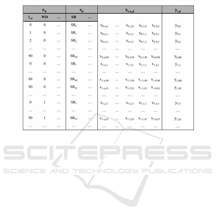
Figure 1: Dataset structure.

3.1.1 Dynamic, Static and Engineered Features

The nature of the features used as input to train ML

models can be distinguished into three main groups

described in the following.

• Static Features (s

): these features are linked

to internal factors of the accommodation facility

recorded for a DOS. They do not change over

time. An example is the starting selling rate,

which is set, for each DOS, at the beginning of

the period that marks the new ﬁnancial business

season for a hotel.

• Dynamic Features (x

t−n,d

): these features change

over time and have been collected both as a varia-

tion from the last recorded value and as an aggre-

gate. An example is given by the number of Room

Nights (RNs) booked on a single day for a DOS

and the number of RNs booked since the ﬁnancial

business season has started up to the considered

day for a DOS.

• Engineered Features (e

): these features are ob-

tained through an engineering process, therefore

resulting from a data transformation process, or

built from scratch. Examples are provided by

the LeadTime column (l

t,d

), which computes the

number of days between the date on which the

prediction is asked and the DOS for which the

prediction is requested, and from the Weekend-

Day column (WD), which indicates if the DOS is

a week-end day or not, and many others.

In addition to the aforementioned features, there is the

target variable (y

t,d

) which is the price dynamically

set by the revenue manager of the receptive structure

as the market conditions, together with the Key Per-

formance Indicators (KPIs) and other factors change.

3.2 Machine Learning Methods

We have performed a benchmark for dynamic price

prediction considering ﬁve machine learning meth-

ods. Speciﬁcally, we have considered a Multiple Lin-

ear Regression (MLR), three models belonging to the

ensemble method with Decision Trees and a Multi-

layer Perceptron (MLP).

• Multiple Linear Regression assumes that a lin-

ear relationship between the dependent variable

and the independent variables exists. It is deﬁned

= β

∑

j=1

i j

+ ε

, (1)

where the β terms are the coefﬁcients to be es-

timated, X are the features related to the model

variables and ε is the model’s error term. The ob-

jective for the MLR is to learn the β terms exploit-

ing training data in order to minimize the residual

Dynamic Price Prediction for Revenue Management System in Hospitality Sector

221

sum of squares between the actual targets and the

ones predicted by the model.

• Ensemble Method with Homogeneous

Learners. The Ensemble method is a learn-

ing technique that combines predictions from

multiple weak learners with the aim of building

a strong learner. The idea under this approach

is that more accurate predictions are obtained

combining different models than those made

by one single model. Since we employed only

decision trees as learners, the ensemble is called

homogeneous. Using decision trees, a distinction

must be made between bagging and boosting

method depending on how the training of the

models in the ensemble is performed (Figure 2).

In our experiments we have used an ensemble

model that is based on bagging, namely the Ran-

dom Forest (RF), and two models based on boost-

ing, i.e., the Gradient Boosting (GB) and the Light

Gradient Boosting (LGB). In RF trees are built

in parallel using bootstrap replicas, obtained by

sampling with replacement. In regression prob-

lems, for a new data point, the model output is

the average of the tree predictions for that point.

In GB and LGB trees are instead built sequen-

tially and additively. These algorithms owe their

name to the use of the gradient descent proce-

dure to minimize the loss function when trees are

added. In particular, after the ﬁrst model is ﬁt-

ted to the training data, the other trees are added

one at a time in order to correct the errors made

by the previous models. The prediction for a new

data point is the sum of the results of each weak

learner contained in the strong learner. What dif-

ferentiates the two models is that in GB trees

are grown level-wise, i.e. giving priority to the

nodes closest to the root, while LGB uses a leaf-

wise strategy, selecting from time to time the leaf

that leads to the most signiﬁcant reduction of the

loss function (Figure 3). Furthermore, LGB em-

ploys two techniques that allows it to be faster

than other boosting models, which are: Gradient-

based One-Side Sampling (GOSS) and Exclusive

Feature Bundling (EFB). The former aims to ﬁl-

ter out data to ﬁnd a split value, by selecting all

records with large gradients and randomly sam-

pling instances with small gradients. The latter is

intended to reduce the complexity of the model

in terms of variables and to speed up the training

phase, by identifying the mutually exclusive vari-

ables, i.e. features which never take on zero value

simultaneously, and grouping them into a single

bundle.

• Multi-layer Perceptron is a feed-forward neural

network, where the data is propagated in only one

direction. It is composed by an input layer, one

or more hidden layers and an output layer (Figure

4). Each neuron in the hidden layers transforms

the values coming from the previous layer with

a weighted linear summation, adds the bias term,

and apply a non-linear activation function.

The model is trained using the backpropagation,

which at each iteration updates the weights of the

network so as to minimize the loss function.

3.3 Evaluation Metrics

To compare the performances of the different mod-

els we have employed the three evaluation measures

described below.

• Mean Absolute Error (MAE): it measures the

average deviation between predictions and actual

values. Consequently, the lower it is the better is

the model. It is deﬁned as

MAE =

∑

i=1

− ˆy

| (2)

where ˆy

is the value predicted by the model,

whereas y

is the target value. Since it uses the ab-

solute value, i.e. it does not consider the direction

of the error, it is a measure that is not sensitive to

extreme values. It is expressed in the same unit of

measure of the target variable, and for this reason

it is a very useful measure for evaluating the per-

formance of various models on a single accom-

modation facility but not for comparing perfor-

mances across hotels. In fact, similar low MAEs

do not necessarily constitute good results in each

case. The goodness of the MAE value must be

evaluated considering the range of the distribution

of the target variable, which clearly differs from

hotel to hotel.

• Mean Absolute Percentage Error (MAPE): it

measures the average percentage of error between

predictions and actual values. It is deﬁned as

MAPE =

100

∑

i=1



− ˆy



, (3)

Like MAE, it is not sensitive to outliers and the

lower the better. It overcomes the highlighted dis-

advantage of MAE because, being expressed as a

percentage, it allows comparison of performances

among hotels.

• Coefﬁcient of Determination: it is also called

, and it measures the goodness of ﬁt of a re-

gression model. It is deﬁned as

= 1 −

∑

i=1

− ˆy

)

∑

i=1

− ¯y

)

(4)

DATA 2024 - 13th International Conference on Data Science, Technology and Applications

222

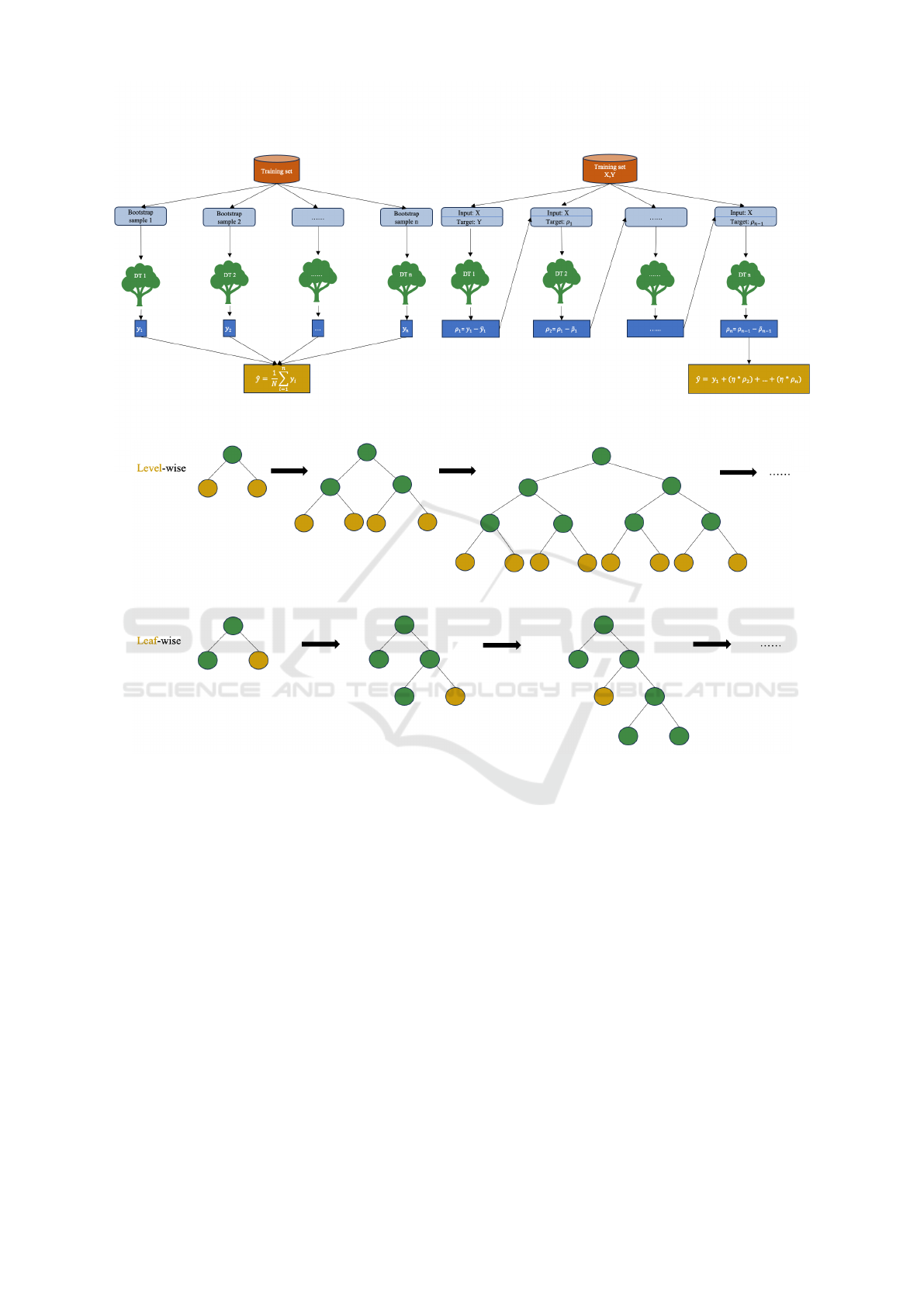
Figure 2: Bagging (left) vs Boosting (right) technique.

Figure 3: Leaf-wise vs level-wise tree growing method.

can take on values between 0 and 1. The

higher, the better. In fact, the higher the value,

the greater the variability in the dependent vari-

able Y expressed by the independent variables X.

This measure therefore also allows us to validate

or deny the logic of the dataset we have built.

4 EXPERIMENTS

This section is dedicated to all aspects related to the

implementation of what has been described so far. We

begin from the presentation of the data collected and

used for the experiments, and then we move on to the

method used to ﬁnd the optimal set of hyperparam-

eters for each machine learning model. We proceed

with the evaluation of the results achieved by the dif-

ferent methods and with the description of the ma-

trix constructed to break down the error into time and

price bands. The last part of this section reports some

consideration regarding the results obtained and the

consequent practical implications.

4.1 Data Collection, Pre-Processing and

Training Details

With the methodology detailed in Section 3, data of

three hotels have been extracted from the database of

a Revenue Management System. Experiments have

been performed for the entry level room of each ac-

commodation facility, where for entry level it is in-

tended the cheapest double room. The reason of this

choice is twofold. First, revenue managers usually set

the selling price for the entry level room and the prices

for all the other rooms are derived from it through a

set of rules. Second, to better evaluate results. In fact,

Dynamic Price Prediction for Revenue Management System in Hospitality Sector

223

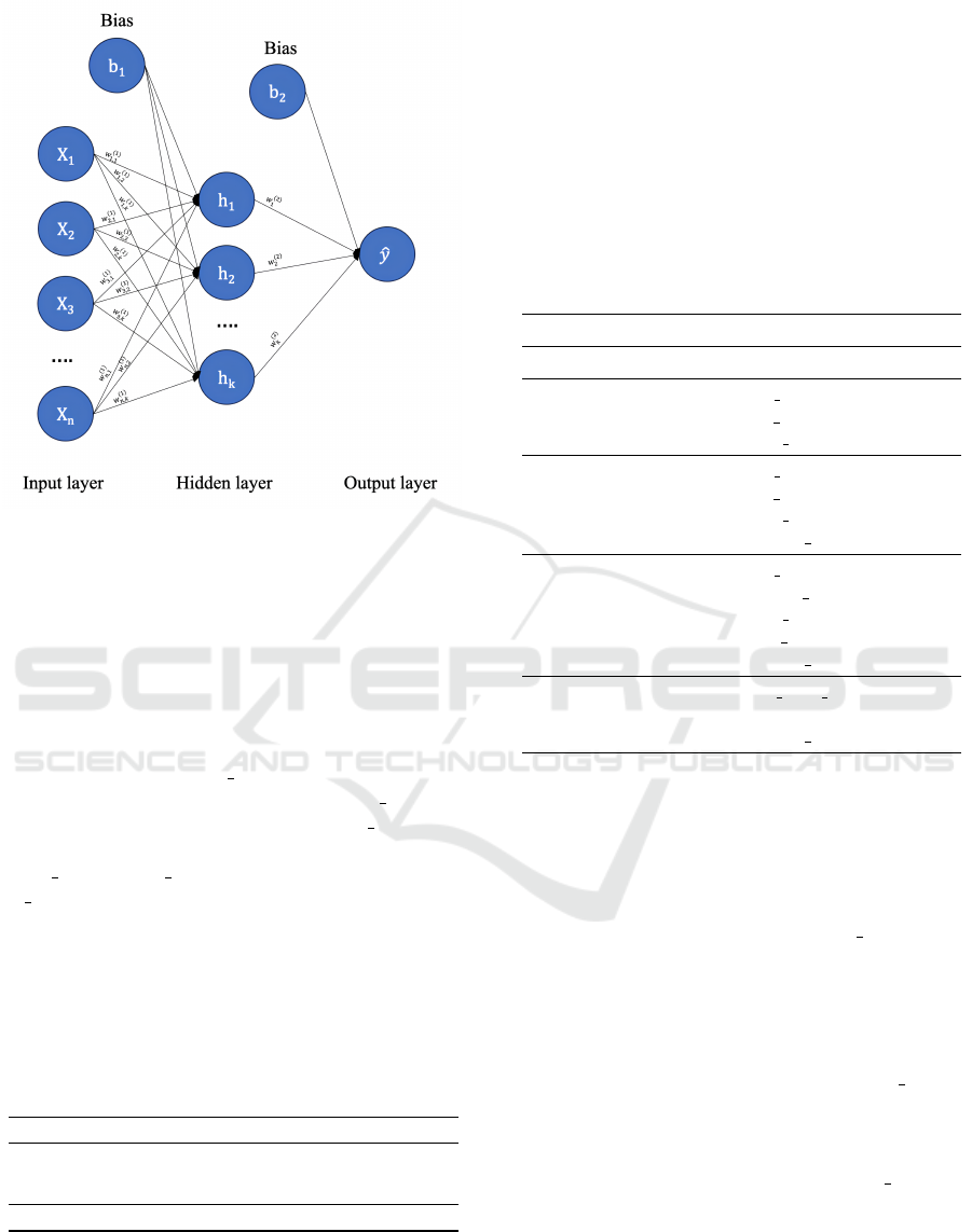
Figure 4: Multi-layer Perceptron structure for regression

tasks.

hotels may have multiple room types with various

prices depending on the room characteristics. Thus, a

way to compare the performance of approaches is to

assess it on “products” that are as similar as possible.

The selected hotels are different in terms of geograph-

ical location, number of available rooms and revenue

manager. Consequently, each hotel has its own dy-

namic price logic. Hotel 1 has 27 operative rooms

(OPRs) of which 17 are entry level. Hotel 2 has 78

OPRs of which 14 are entry level. Hotel 3 has 107

OPRs of which only 10 are entry level. Moreover,

Hotel 1 and Hotel 2 are located in Italy, while Ho-

tel 3 is based in Switzerland. After being collected,

data of each hotel have been pre-processed and di-

vided into training, validation and test set. The set of

data of each hotel contains a total of 59423 samples,

covering the period from 1

of January 2022 to 15

of October 2023. Table 1 reports details related to the

split for each set of data.

Table 1: Training, validation and test sets for each hotel.

SET PERIOD N° OF SAMPLE

Training from 2022/01/01 to 2022/12/31 33215

Validation from 2023/01/01 to 2023/05/31 13741

Test from 2023/06/01 to 2023/10/15 12467

TOT. Samples 59423

Since each hotel has its own dynamic pricing strat-

egy, the hyperparameters required by each Machine

Learning model has been set on a per-hotel basis. For

this purpose, we have picked out for every model the

hyperparameters to be optimized (shown in Table 2)

and, for each of these, we have deﬁned a zone of in-

terest, i.e., the possible values they can took on. We

have subsequently carried out a grid search to ﬁnd

the best set of hyperparameters per model per hotel,

where ”best” means that values that minimize or max-

imize our evaluation measures (i.e., MAE, MAPE and

) have been chosen. This step has been performed

by looking at the results on the validation sets.

Table 2: Hyperparameters optimized with a grid search for

the compared models.

MODEL HYPERPARAMETERS OPTIMIZED

MLR positive

RF n trees

max features

max depth

GB n trees

max features

max depth

learning rate

LGB n trees

colsample bytree

max depth

num leaves

learning rate

MLP hidden layer size

solver

learning rate

4.2 Results

Table 3 reports the performances of the different ma-

chine learning models on the test sets of the three ho-

tels. For a better evaluation of the results, the predic-

tions and actual values related to Hotel 3 have been

converted from Swiss francs into euros considering

the currency existing at the time of the experiments,

i.e., 1.04 Swiss francs for 1 euro. Looking at the re-

sults, it can be observed that there is no model that

clearly prevails over the others: Light Gradient Boost-

ing (LGB) provides the best results for Hotel 1 while

for the other two receptive structures it seems that

Multiple Linear Regression (MLR) is better. Compar-

ing the performances across hotels, the signiﬁcantly

better performance was obtained for Hotel 3, with a

MAPE of 0.3771 and an R

of 0.9662.

Since we deal with a dynamic pricing strategy,

it is important to discern the error and understand if

there is a time horizon and/or a price range in which

the model produces worse performances and detect

for possible reasons. To this end, the test data sets

have been divided into four time horizons (H

) and

DATA 2024 - 13th International Conference on Data Science, Technology and Applications

224

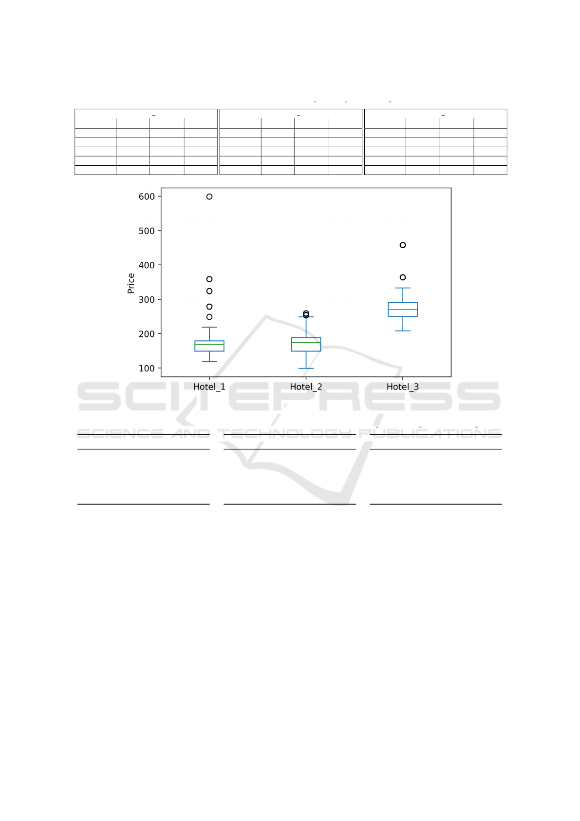
Table 3: Results on test sets for Hotel 1, Hotel 2 and Hotel 3.

Hotel 1

MODEL MAE MAPE R

MLR 3.1820 1.9087 0.9189

RF 2.5146 1.4629 0.9232

GB 1.9479 1.1307 0.9240

LGB 1.8845 1.1000 0.9340

MLP 2.7272 1.6201 0.9182

Hotel 2

MODEL MAE MAPE R

MLR 3.4445 2.0197 0.9037

RF 6.7323 3.4384 0.8423

GB 5.9982 3.2247 0.8429

LGB 5.9894 3.1863 0.8343

MLP 3.5753 2.1117 0.9080

Hotel 3

MODEL MAE MAPE R

MLR 0.9380 0.3771 0.9662

RF 1.8742 0.7391 0.9112

GB 1.7649 0.7051 0.9124

LGB 1.7659 0.6711 0.8676

MLP 1.0482 0.4136 0.9650

Figure 5: Boxplot of the test set price distribution per hotel.

Table 4: Statistical indexes computed on the test set for the target variable for Hotel 1 (a), Hotel 2 (b) and Hotel 3 (c).

STATISTICAL INDEX VALUE

Max 599

75 p. 179

50 p. 169

25 p. 149

Min 119

(a)

STATISTICAL INDEX VALUE

Max 259

75 p. 189

50 p. 174

25 p. 149

Min 99

(b)

STATISTICAL INDEX VALUE

Max 458

75 p. 291

50 p. 270

25 p. 250

Min 208

(c)

four price bands (B

). To identify the ideal splits for

the prediction horizons we have consulted the domain

experts and set the following periods:

: predictions from 0 to 7 days ahead.

: predictions from 8 to 15 days ahead.

: predictions from 16 to 30 days ahead.

: predictions from 31 to 90 days ahead.

Since the distribution of prices in the test sets differs

even considerably among hotels (see boxplots in Fig-

ure 5), it would not have been possible to arbitrarily

create four price ranges. For this reason, we decided

to make use of the main statistical indices (shown in

Table 4) together with a criterion applicable regard-

less of the distribution of the prices. We used the min-

imum value, the 25

, the 50

and the 75

percentile

and the maximum value of each distribution to split

prices, obtaining the following bands:

: prices between the minimum value and the

percentile.

: prices greater than the 25

percentile and less

than or equal to the 50

percentile.

: prices greater than the 50

percentile and less

than or equal to the 75

percentile.

: prices greater than the 75

percentile and less

than or equal to the maximum price.

By considering the time horizons and the price bands,

we have computed matrices to highlight the MAPE

for each horizon-price combination (Figure 6).

Dynamic Price Prediction for Revenue Management System in Hospitality Sector

225

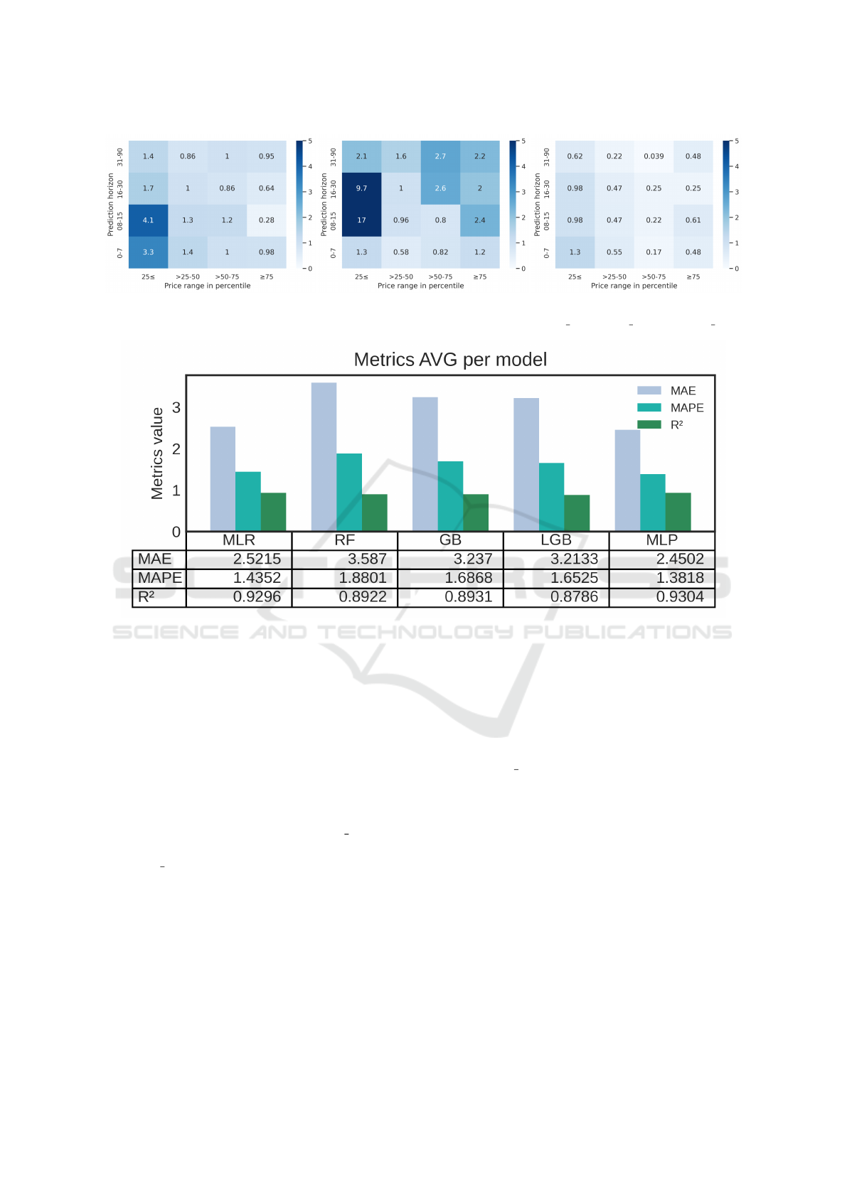
(a) (b) (c)

Figure 6: Matrices with MAPE over the ﬁxed temporal horizons and price bands for Hotel 1 (a), Hotel 2 (b) and Hotel 3 (c).

Figure 7: Bar chart and table with the average of MAE, MAPE and R

computed on the performances of the three hotels per

each model, MLR, RF, GB, LGB and MLP.

4.3 Discussion and Implications

Although the best performing models are LGB and

MLR as shown in Table 3, the model that allows for

an overall lower average error is the MLP, as shown in

Figure 7. From a practical point of view, this implies

that if an RMS wish to implement a single model for

all the accommodation facilities, MLP is to be pre-

ferred among the ones compared in this study.

Another consideration concerns Hotel 2. As can

be seen, looking at the results in Table 3 and Figure

6b, Hotel 2 is the receptive structure with the high-

est errors in terms of MAE and MAPE. It has also

the lowest coefﬁcient of determination. We hypothe-

sized that this behavior could be linked to the fact that

this property has changed its revenue manager starting

from the 1

of May of 2023. This means that the pre-

dictions have been obtained based on models trained

on the pricing strategy of the previous domain expert

and tested on the pricing strategy of the new domain

expert. Despite this, the results are still satisfactory

and, in these cases, we should simply give the model

time to adapt and learn the new strategy. Our hypoth-

esis could also be conﬁrmed by the fact that while

for the other two hotels the results on the test set are

slightly better than those obtained on the validation

set, for Hotel 2 there is instead a worsening of 1.0323

in MAE and 0.4218 in MAPE. It should be speciﬁed

that although the validation set has been used to tune

the hyperparameters, we are not surprised by the fact

that we got small improvements on the test set. We

supposed that these are linked to the period tested; in

fact, the test set covers the summer season in which

sales price changes are usually more frequent, and

therefore the model may have learned better because

it have had more relevant examples in the training set.

Lastly, observing the average percentage error matri-

ces in Figure 6 it can be noted that the highest errors

are more concentrated in the B

price band and ap-

proximately in the H

and H

time horizons. One of

the possible explanations could be that we are not tak-

ing into account some variables that are closely linked

DATA 2024 - 13th International Conference on Data Science, Technology and Applications

226

to bookings that take place between 0 and 15 days be-

fore the DOS, i.e., meteorological variables. In fact,

when the price is lower than normal, weather condi-

tions can be decisive in the choice to make a reserva-

tion or not.

5 CONCLUSIONS AND FUTURE

WORKS

In this study we have performed a benchmark of dif-

ferent machine learning methods with the aim to build

a support useful for a revenue manager working on

dynamic prices. Having a well-established dynamic

pricing strategy, the continuous monitoring and man-

ual adjustment of prices performed by a revenue man-

ager becomes costly and time-consuming. For this

purpose we built a dataset containing static, dynamic

and engineered variables and applied ﬁve machine

learning models, MLR, RF, LGB, GB and MLP to

predict the dynamic price that a revenue manager

would set every day for the next 90 days for the entry

level room of a receptive structure. The approaches

have been tested on three different hotels. Since it

emerged that the highest errors in terms of MAPE

are concentrated more in the predictions between 0-

15 days and in the lowest price range, in future works

we will try to exploit additional variables that could

inﬂuence the decision of the price in these cases.

REFERENCES

Abrate, G., Nicolau, J. L., and Viglia, G. (2019). The impact

of dynamic price variability on revenue maximization.

Tourism Management, vol. 74, pp. 224-233.

Al Shehhi, M. and Karathanasopoulos, A. (2020). Forecast-

ing hotel room prices in selected gcc cities using deep

learning. Journal of Hospitality and Tourism Manage-

ment, vol. 42, pp. 40-50.

Alshakhsheer, F., Habiballah, M., Al-Ababneh, M. M., and

Alhelalat, J. A. (2017). Improving hotel revenue through

the implementation of a comprehensive dynamic pricing

strategy: A conceptual framework and empirical inves-

tigation of jordanian hotels. Business Management Dy-

namics, vol. 7, pp.19-33.

Bandalouski, A. M., Egorova, N. G., Kovalyov, M. Y.,

Pesch, E., and Tarim, S. A. (2021). Dynamic with

demand disaggregation for hotel revenue management.

Journal of Heuristics.

Bayoumi, A., Saleh, M., Atiya, A., and Habib, H. (2013).

Dynamic pricing for hotel revenue management using

price multipliers. Journal of Revenue and Pricing Man-

agement.

Deksnyte, I. and Lydeka, Z. (2012). Dynamic pricing and its

forming factors. Journal of Business and Social Science.

El-Nemr, N., Canel-Depitre, B., and Taghipour, A. (2019).

Determinants of hotel room rates determinants of hotel

room rates. In Luxury Industries Conference.

Elreedy, D., Atiya, A. F., Fayed, H., and Saleh, M. (2019).

A framework for an agent-based dynamic pricing for

broadband wireless price rate plans. Journal of Simu-

lation, vol. 13, pp. 96-110.

Goli, F. and Haghighinasab, M. (2022). Dynamic pricing: A

bibliometric approach. Iranian Journal of Management

Studies, vol. 15, pp. 111-132.

Kalehbasti, P., Nikolenko, L., and Rezaei, H. (2019).

Airbnb price prediction using machine learning and sen-

timent analysis. In CD-MAKE, International Cross-

Domain Conference for Machine Learning and Knowl-

edge Extraction.

Lak, P., Kocak, A., Pralat, P., Bener, A., and Samarikhalaj,

A. (2015). Towards dynamic pricing for digital billboard

advertising network in smart cities. In ISC2, IEEE First

International Smart Cities Conference.

Liu, Y. (2021). Airbnb pricing based statistical machine

learning models. In CONF-SPML, International Confer-

ence on Signal Processing and Machine Learning.

Mariani, M. and Wirtz, J. (2023). A critical reﬂection

on analytics and artiﬁcial intelligence-based in analytics

in hospitality and tourism management research. Inter-

national Journal of Contemporary Hospitality Manage-

ment, vol. 35, pp. 2929-2943.

Pande, R. (2020). Investigation of the implementation of

machine learning within the hospitality industry. In

CAUTHE Conference.

Peng, N., Qin, Y., and Li, K. (2020). Leveraging multi-

modality data to airbnb price prediction. In ICEMME,

International Conference on Economic Management

and Model Engineering.

Ragapriya, N., Kumar, T. A., Parthiban, R., Divya, P., Jay-

alakshmi, S., and Raman, D. R. (2023). Machine learn-

ing based house price prediction using modiﬁed extreme

boosting. AHAST, Asian Journal of Applied Science and

Technology.

Sahin, M. (2019). Optimization of dynamic ticket pricing

parameters. Journal of Revenue Pricing Management,

vol. 18, pp. 306-316.

Sahin, M. and Erol, R. (2017). A dynamic ticket pricing

approach for soccer games. Axioms, vol. 6.

Shadiqurrachman, S., Ridwan, A. Y., and Kusuma, A.

(2019). Online travel agency channel pricing policy

based on dynamic pricing model to maximize sales

proﬁt using nonlinear integer programming approach. In

ICOEMIS, Proceedings of the 1st International Confer-

ence on Engineering and Management in Industrial Sys-

tem.

Shakya, S., Kern, M., Owusu, G., and Chin, C. M. (2012).

Neural network demand models and evolutionary opti-

misers for dynamic pricing. In 13th SGAI International

Conference on Innovative Techniques and Applications

of Artiﬁcial Intelligence.

Shehhi, M. A. and Karathanasopoulos, A. (2018). Forecast-

ing hotel prices in selected middle east and north africa

region (mena) cities with new forecasting tools. Theoret-

ical Economics Letters, vol. 8, pp. 1623-1638.

Shintani, M. and Umeno, K. (2022). General dynamic pric-

ing algorithms based on universal exponentialn booking

Dynamic Price Prediction for Revenue Management System in Hospitality Sector

227

curves. JSIAM Letters, vol. 14, pp. 49-52.

Vives, A. and Jacob, M. (2020). Dynamic pricing for on-

line hotel demand: the case of resort hotels in majorca.

Journal of Vacation Marketing, vol. 26, pp. 1-16.

Vives, A. and Jacob, M. (2021). Dynamic pricing in differ-

ent spanish resort hotels. Journal of Tourism Economics,

vol. 27, pp. 1-14.

Vives, A., Jacob, M., and Aguil

o, E. (2019). Online hotel

demand model and own-price elasticities: An empirical

application to two resort hotels in a mature destination.

Tourism Economics, vol. 24, pp. 720-752.

Ye, P., Qian, J., Chen, J., Wu, C., Zhou, Y., De Mars, S.,

Yang, F., and Zhang, L. (2018). Customized regres-

sion model for airbnb dynamic pricing. In 24

ACM

SIGKDD International Conference on Knowledge Dis-

covery & Data Mining.

Zhang, Q., Qiu, L., Wu, H., Wang, J., and Luo, H. (2019).

Deep learning based dynamic pricing model for hotel

revenue management. In ICDMW, International Confer-

ence on Data Mining Workshops.

Zhang, Z., Chen, R. J. C., Han, L. D., and Yang, L. (2017).

Key factors affecting the price of airbnb listings: A geo-

graphically weighted approach. Sustainability, vol. 9.

Zhu, F., Xiao, W., Yu, Y., Wang, Z., Chen, Z., Lu, Q. Liu, Z.,

Wu, M., and Ni, S. (2022). Modeling price elasticity for

occupancy prediction in hotel dynamic pricing. In Pro-

ceedings of the 31st ACM International Conference on

Information & Knowledge Management, pp. 4742-4746.

DATA 2024 - 13th International Conference on Data Science, Technology and Applications

228