Utilizing Sensor and Actuator Virtualization to Achieve a Systemic View
of Mobile Heterogeneous Cyber-Physical Systems
Martin Richter
1
, Reinhardt Karnapke
2
and Matthias Werner
1
1
Operating Systems Group, Chemnitz University of Technology, Germany
2
Chair of Distributed Systems/Operating Systems, Brandenburg University of Technology, Germany
Keywords:
Cyber-Physical Systems, Virtualization, Mobility, Heterogeneity, Transparency.
Abstract:
When programming cyber-physical systems, application developers currently utilize physical sensors and ac-
tuators individually to achieve the desired observations and impacts within the physical world. This is an
error-prone and complex task given the size, heterogeneity, and mobility of prevailing cyber-physical sys-
tems. We introduce an application model that allows the application developers to take a physical perspective.
By means of this model, the programmers describe desired observations and influences with respect to the
physical world without directly referencing physical devices. We present an additional model for a runtime
environment that transparently utilizes the available physical devices to reach the application developers’ tar-
gets. We show that an implementation of our models is functional via simulation.
1 INTRODUCTION
Cyber-Physical Systems (CPS) play an ever-
increasing role because of trends like the Internet
of Things and Industry 4.0. Such systems observe
and influence their physical environment via sensors
and actuators. These devices are distributed through
space and may be heterogeneous as well as mobile.
Classically, the application developers program these
devices individually to achieve a desired impact on
the physical world. This alone, is an error-prone and
complex task under the mentioned circumstances due
to explicit communication between and coordination
of the devices. Adding to this, it is the standard
for programmers to take a digital perspective when
programming such systems. This makes the desired
impact on the environment less clear, as control
and measurement signals may not reflect physical
circumstances accurately. For example, the input
signal for a light actuator can be represented either
by ON or OFF while the resulting illumination is not
clear from setting this signal.
We argue that with the decreasing costs of com-
putation units and their increasing processing power,
more sophisticated models should be employed. We
introduce an application model that allows the appli-
cation developers to take a physical perspective when
programming CPS. It allows them to describe the
properties of physical phenomena of interest and how
these properties should evolve over time. This makes
the desired impact of the application on the environ-
ment clear. Complementing this application model,
we introduce a Runtime Environment (RTE) that sup-
ports the interpretation of the application program-
mers’ descriptions. Based on these descriptions the
RTE utilizes the available physical sensors and actua-
tors transparently with respect to the application. We
achieve this by integrating device virtualization into
the RTE. We define virtualization as the deployment
of a virtual device that, during runtime, is mapped
onto (possibly multiple) physical devices on demand.
Our model refers to virtual sensors and actuators that
represent the capabilities to observe and influence the
applications’ phenomena of interest. During runtime,
each virtual device utilizes varying sets of physical
devices based on their capabilities to achieve the de-
sired observation or influence of the physical phe-
nomena of interest. As a consequence, the application
is detached from directly interacting with the physical
devices. This in conjunction with programming from
the physical perspective allows the developers to take
a systemic view that is independent from changing
sets of mobile and heterogeneous physical devices.
Thus, distribution transparency is achieved and the
programmers are able to focus on their targets with
respect to the physical environment.
The remainder of this paper is structured as fol-
lows. Section 2 presents related work focussing on
Richter, M., Karnapke, R. and Werner, M.
Utilizing Sensor and Actuator Virtualization to Achieve a Systemic View of Mobile Heterogeneous Cyber-Physical Systems.
DOI: 10.5220/0012715800003758
Paper published under CC license (CC BY-NC-ND 4.0)
In Proceedings of the 14th International Conference on Simulation and Modeling Methodologies, Technologies and Applications (SIMULTECH 2024), pages 207-214
ISBN: 978-989-758-708-5; ISSN: 2184-2841
Proceedings Copyright © 2024 by SCITEPRESS – Science and Technology Publications, Lda.
207

sensor and actuator virtualization for CPS. In Sec-
tion 3, we provide a running example for illustrative
purposes. Section 4 contains the theoretical concept
of our approach and presents an initial evaluation.
Section 5 provides a conclusion and an outlook on the
next steps to take.
2 RELATED WORK
Existing operating systems for robotic systems, such
as the Robot Operating System 2 (ROS 2) (Macenski
et al., 2022) or XBot2 (Laurenzi et al., 2023), are fun-
damentally suited for deployment in CPS. Though
these operating systems provide basic abstractions
for utilizing various individual devices, they lack the
transparent utilization of sets of devices that our vir-
tualization model offers.
In (Tsiatsis et al., 2010), an architecture is intro-
duced that utilizes a resource layer. This layer ab-
stracts from individual physical devices and provides
a uniform interface for accessing them. Apart from
this interface, the developers have to specify which
sensors and actuators are to be employed. This re-
quires explicit knowledge of the capabilities of the
devices. As a result, the application is still directly
bound to physical sensors and actuators.
In (Suh et al., 2013), a similar concept is pre-
sented. It enables the developers to select physi-
cal sensors and actuators based on their capabilities
and the contexts they are located within. After the
programmers select the devices, they have to con-
trol them explicitly. Therefore, no virtualization is
achieved which inhibits transparently utilizing mul-
tiple different sensors and actuators.
In (Fernandez-Cortizas et al., 2023), an approach
to software synthesis is presented that transforms an
application into a behavioral plan consisting of multi-
ple actions. Before runtime, this plan is distributed
among the various physical devices based on their
capabilities. Each device possesses its own imple-
mentation of the different actions. As the distribu-
tion of tasks is performed before runtime, no dynamic
task allocation is possible and changing environmen-
tal factors cannot be taken into account.
In (Vicaire et al., 2010a) and (Vicaire et al.,
2010b), the concept of Bundles is introduced. It en-
ables the developers to define groups of physical de-
vices that are utilized for the execution of the appli-
cation. Each group is identified by an abstract de-
vice type (e.g., cameras). The group membership of
a device may change during runtime based on chang-
ing conditions (e.g., motion). The devices within the
group are managed individually by the developers.
Consequently, there is no virtualization support for
heterogeneous devices.
In (Ni et al., 2005) and (Borcea et al., 2004), a
similar approach is chosen. The application selects
devices based on their location and capabilities. After
selection, the developers manage sensors and actua-
tors individually which is in conflict with a transpar-
ent utilization of multiple physical devices.
In (Seiger et al., 2015), ROS 2 is extended by
an abstraction layer that focuses on the uniform pro-
gramming of home robots. Each of these robots may
possess different abstract capabilities (e.g., grab or
move). The robots may implement these capabili-
ties differently based on their available sensors and
actuators. The application utilizes abstract capabili-
ties to describe the desired behavior of a robot. As
the robots are programmed individually the concept
neither provides distribution transparency nor virtual-
ization of multiple devices.
In (Beal and Bachrach, 2006), an approach is pre-
sented that allows programmers to develop applica-
tions with respect to continuous regions in space. A
virtual device is present at each location within these
regions. Every virtual device provides measurements,
processing power, and actuation. The execution of
the application is then approximated by a discrete set
of physical devices that are located within the region.
Each of these devices executes the same application
code. This code consists of operations that refer to
the local state of the executing node as well as the
states of nodes in its proximity. This allows the de-
velopers to take a systemic view but limits the system
to a homogeneous set of devices.
It is evident from the discussed concepts that
existing approaches focus on making physical de-
vices more accessible for application programmers.
Though this takes away complexity from developing
applications for CPS, key challenges like the utiliza-
tion of multiple heterogeneous physical devices re-
main open.
3 RUNNING EXAMPLE
This section presents a running example that shows
the strengths of our approach with respect to the de-
tachment of the application programmers from the
utilized physical devices.
The example comprises a factory scenario in
which light-sensitive products are fabricated in a se-
ries of steps. Each step takes place in a different fac-
tory hall. Hallways connect the buildings and au-
tonomous robots move the products between them.
These robots avoid regions exposed to light by uti-
SIMULTECH 2024 - 14th International Conference on Simulation and Modeling Methodologies, Technologies and Applications
208

lizing brightness sensors. To keep their path planning
as efficient as possible, light sources should be turned
off within the factory during production. This can-
not generally be guaranteed as human workers irreg-
ularly and sparsely have to perform maintenance on
the fabrication machines. The application in this sce-
nario comprises the lighting control within the fac-
tory such that working conditions are safe for humans
while influences on the products are minimized. This
encompasses individually turning lights on or off de-
pending on where people are present. To identify peo-
ple within the factory, the application may utilize in-
formation from security cameras as well as from the
employed robots (e.g., attached infrared cameras and
distance sensors).
Our virtualization model allows the application
developers to focus on describing their target, i.e., a
desired observation of and influence on the physical
environment. Transparent to the application, the RTE
handles the technical details for utilizing the required
devices (e.g., the available cameras, lighting, robots,
and their positioning). The running example encom-
passes mobility and heterogeneity of devices, physi-
cal phenomena, as well as different physical contexts
that restrict the capabilities of physical sensors and
actuators. Thus, it is well suited for presenting the
capabilities of our virtualization model.
4 CONCEPT
As described in Section 1, the developers take a phys-
ical perspective such that a systemic view is accom-
plished. The following sections introduce an environ-
mental model and an application model to describe
the programmers’ view on the physical environment.
Based on these models, we introduce an approach to
I/O-device virtualization. It connects the application
and the physical devices that influence and observe
physical phenomena.
4.1 Environmental Model
The developers create an application for observing
and influencing a physical phenomenon of interest P
within the physical system Σ. The system region is
denoted X
Σ
and represents the developers’ space of
interest within which the physical phenomenon may
reside (e.g., a factory comprised of different produc-
tion halls and hallways). Multiple properties charac-
terize such a phenomenon (e.g., the shape of a hu-
man and the brightness around it). These properties
represent the phenomenon’s state ⃗z and may change
over time t. The change of state
˙
⃗z represents the
phenomenon’s behavior. It is composed of an inter-
nally induced change
˙
⃗z
int
and an externally induced
change
˙
⃗z
ext
. The function
˜
f represents their composi-
tion:
˙
⃗z(t) =
˜
f (
˙
⃗z
int
(t),
˙
⃗z
ext
(t)). Internal factors resem-
ble a change of state
˙
⃗z
int
based on the phenomenon’s
current state ⃗z (e.g., an object changing its position
due to its current velocity). External factors refer to
changes
˙
⃗z
ext
induced by controlled activities of actu-
ators (e.g., an object changing its position due to a
robot applying force to it). Control signals ⃗u induce
these actuator activities. The function f describes the
behavior of the phenomenon based on its current state
⃗z and the actuator control signals ⃗u (similar to control
theory):
˙
⃗z(t) = f (⃗z(t),⃗u(t)).
Sensors S provide information on the properties
of a phenomenon by measuring physical quantities q
(e.g., a camera measures electromagnetic radiation).
Actuators A influence these properties by inducing
changes ˙q in physical quantities, (e.g., a light source
illuminates its environment). Sensors and actuators in
conjunction form the available physical I/O devices D
within the system. This set may change over time due
to devices joining or leaving the system (e.g., due to
failure and repair). In (Richter et al., 2023) we intro-
duced a physical context model for sensors. The same
model is applicable to actuators as well. It allows to
infer how the outputs of devices may be utilized with
respect to their capabilities and the physical contexts
they reside in. The model associates with each device
d a class ζ, a context region X
c
(d), an effective output
region X
e f f
(d), an associated physical quantity d.q,
and a location d.⃗x.
4.2 Application Model
As described in Section 1, the developers write the ap-
plication from a physical point of view. It is their goal
to determine sufficient external influences on physi-
cal phenomena of interest, such that these phenom-
ena reach a target state. Therefore, their application is
composed of a phenomenon description. Such a de-
scription consists of a state description vector
⃗
ρ that
allows to observe the physical phenomenon’s state ⃗z
based on interpretations of available sensor measure-
ments, and a behavioral function b that determines
the required external state influences
˙
⃗z
ext
that alter the
state of the phenomenon over time via actuator ac-
tivities while taking the phenomenon’s internal state
changes into account.
The state description vector
⃗
ρ provides the
information necessary for discriminating different
phenomena. Each of its elements is a tuple, consisting
of a type τ
i
and a rule r
i
. A type ρ
i
.τ represents a set of
possible values for the property. A rule ρ
i
.r is a func-
Utilizing Sensor and Actuator Virtualization to Achieve a Systemic View of Mobile Heterogeneous Cyber-Physical Systems
209

tion that equals one if a value of type τ
i
characterizes
the phenomenon (e.g., the shape of an object should
resemble a human). Within the physical system,
possibly multiple phenomena P = {P
1
...P
m
} may
be present that suffice the description
⃗
ρ. The follow-
ing equation describes this: ∀P
i
∈ {P
1
,...P
m
} :
⃗z
P
i
(t) =

z
P
i
,1
(t) . . . z
P
i
,n
(t)

T
,z
P
i
, j
(t) ∈
ρ
j
.τ, ρ
j
.r(z
P
i
, j
(t)) = 1, j ∈ [1, n]. The RTE
transparently utilizes a function g to instantiate the
state vectors ⃗z
P
i
for each observed phenomenon that
suffices the state description vector. This function
interprets the outputs of the available sensors S(t)
based on the state description
⃗
ρ while taking the
sensors’ related output and context regions into
account. This allows determining values for the
different state variables as well as calculating the
spatial regions X
P
i
in which the phenomena reside,
i.e.,

(⃗z
P
1
(t), X
P
1
(t)) . . . (⃗z
P
m
(t), X
P
m
(t))

T
=
g(S(t),
⃗
ρ), P
j
∈ P.
For describing how a target phenomenon state
should be reached, the application programmers de-
velop the behavioral function b. Its inputs are pro-
vided by the RTE and are composed of the measured
state vector ⃗z
P
i
that allows the application to con-
sider internal state changes, and a set of currently
available external state influences
˙
⃗z
P
i
,ext
that enable
the application to choose a vector of desired influ-
ences
˙
⃗z
P
i
,ext
from them to reach a target state such
that
˙
⃗z
P
i
,ext
(t) = b(⃗z
P
i
(t),
˙
⃗z
P
i
,ext
(t)),
˙
⃗z
P
i
,ext
(t) ∈
˙
⃗z
P
i
,ext
(t).
The phenomenon may reach a target state without any
outside influences (i.e., due to internally induced state
changes). Therefore, the application developers have
to take the current state⃗z
P
i
,ext
of the phenomenon and
its internally induced state changes (that are deducible
from its current state) into account. Under these con-
siderations, by applying b they select an externally in-
duced state change
˙
⃗z
P
i
,ext
from the available externally
inducible state changes
˙
⃗z
P
i
,ext
.
The RTE calls the behavioral function b of the
corresponding phenomenon description for each iden-
tified state vector ⃗z
P
i
. The RTE transparently de-
termines the currently available externally inducible
state changes via a function h based on the currently
available actuators A and the region X
P
i
in which
the phenomenon instance resides, i.e.,
˙
⃗z
P
i
,ext
(t) =
h(A(t), X
P
i
(t)). Taking the phenomenon’s region into
account is necessary as the effective output regions of
actuators (see Section 4.1) have to intersect the phe-
nomenon’s region to influence it. Based on the re-
sult
˙
⃗z
P
i
,ext
, the RTE transparently utilizes a function
¯
h to determine sufficient actuator inputs ⃗u
P
i
for the
available actuators A to influence the state of phe-
nomenon P
i
. This is summarized by the equation
⃗
ρ =


(τ
1
,r
1
)
.. .
(τ
n
,r
n
)


˙
⃗z
P
1
,ext
= b(⃗z
P
1
,
˙
⃗z
P
1
,ext
)
.. .
˙
⃗z
P
m
,ext
= b(⃗z
P
m
,
˙
⃗z
P
m
,ext
)
Application
g
⃗
ρ
{⃗z
P
i
}
h
{X
P
i
}
{
˙
⃗z
P
i
,ext
}
¯
h
{
˙
⃗z
P
i
,ext
}
Sensors
Actuators
P = {P
1
,. . . , P
m
}
Physical Environment
S
{⃗u
P
i
}
A
q
1
,q
2
,. . .
˙q
1
, ˙q
2
,. . .
RTE
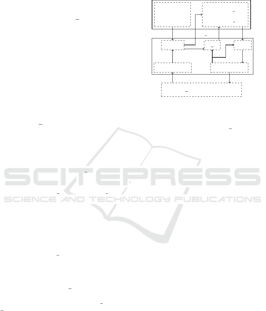
Figure 1: Depiction of the application model, consisting of
a state description
⃗
ρ and a behavioral function b for a phe-
nomenon P of which multiple instances P
i
may be present;
including the interface to the RTE (i.e., g, h, and
¯
h).
⃗u
P
i
(t) =
¯
h(A(t),
˙
⃗z
P
i
,ext
(t)). Figure 1 depicts our ap-
plication model in conjunction with the described in-
terfaces to the RTE.
The presented model enables the application de-
velopers to describe desired influences on physical
phenomena. Depending on the application, there may
be a need for a default behavior, i.e., developers spec-
ifying desired influences on the environment for loca-
tions at which the phenomenon is not observed. In our
running example, this refers to lights being turned off
at all locations with no worker being present. This de-
fault behavior is not dependent on any state descrip-
tion. Rather, it specifies a behavior for all locations
that is then overwritten by the behavior of observed
non-default physical phenomena at their respective
locations. This overwriting is performed by the RTE
based on priorities that the application developers as-
sign to the behavior of phenomena. From the appli-
cation’s perspective, the developers achieve this de-
fault behavior by specifying a physical phenomenon
with no state description (i.e., by only specifying the
behavioral function b). Such a default phenomenon
represents a phenomenon for which all available state
changes may be relevant.
Listing 1 depicts this for our running example in
Python code. In the main function, the developers ini-
tialize the RTE by making the phenomena of inter-
est (i.e., Default and Person) known. The Default
phenomenon specifies that from all available inputs
in all locations, the ones that provide a minimum
brightness should be chosen (i.e., lights being turned
off). The Person phenomenon encompasses a state
description and a behavior description. The state de-
SIMULTECH 2024 - 14th International Conference on Simulation and Modeling Methodologies, Technologies and Applications
210

scription specifies that the phenomenon possesses the
shape of a human and that the brightness around it is
of relevance (although no direct rule is given as a per-
son should be identified independent of the brightness
around it). The behavioral function specifies that from
all available property changes that may influence the
person, the one that provides the minimum brightness
above the required working conditions of 250 Lumen
should be chosen. The priorities P_MIN and P_MAX are
assigned such that the default phenomenon is over-
written wherever a person is identified. It is now the
task of the RTE to identify these phenomena of inter-
est, determine available influences on them, call the
behavioral functions of the instantiated phenomena,
and realize the resulting desired influences.
impo r t r t e
from p r i o r i t i e s impo r t P MIN , P MAX
from p r o p e r t i e s i mpor t B r i g h t n e s s , S hape
from p r o p e r t i e s i mpor t D e f a u l t P h e n , P h y s i c a l P h e n
c l a s s D e f a u l t ( D e f a u l t P h e n ) :
d e f p r i o r i t y ( ) : r e t u r n P MIN
d e f b e h a v i o r ( , c h a n g e s ) :
i f ” B r i g h t n e s s ” no t i n c h a n g e s : r et u r n {}
r e t ur n { ” B r i g h t n e s s ” : min ( c h a n g e s [ ” B r i g h t n e s s ” ] ) }
c l a s s P e r s o n ( P h y s i c a l P h e n ) :
d e f p r i o r i t y ( ) : r e t u r n P MAX
d e f s t a t e ( ) : r e t u r n {” B r i g h t n e s s ” : ( lambda b : Tr ue ) ,
” S h ape ” : ( lambda s : s == Sha p e . human ) }
d e f b e h a v i o r ( s t a t e , c h a n g e s ) :
i f s t a t e [ ” B r i g h t n e s s ” ] > =250: # Lumen
r e t ur n {}
i f ” B r i g h t n e s s ” no t i n c h a n g e s : r et u r n {}
c h o se n = [ c f o r c i n c h a n g e s [ ” B r i g h t n e s s ” ] i f c >=250]
i f c h o s e n = = [ ] : r e t u rn {}
r e t ur n { ” B r i g h t n e s s ” : min ( c h o s e n )}
d e f ma in ( ) :
r t e . i n i t i a l i z e ( [ P e r s on , D e f a u l t ] )
Listing 1: Python code for the application implementing the
desired behavior of our running example (see Section 3).
4.3 Runtime Environment
As described in Section 1, we define virtualization
as the transparent provision of a virtual device that
is mapped onto physical devices at access or on de-
mand. Based on the application’s target, a virtual de-
vice dynamically merges the capabilities of possibly
multiple physical devices. In our application model,
the functions g, h, and
¯
h represent this abstractly.
These functions respectively aggregate and dissemi-
nate information according to the application’s goal
and the available physical devices. To realize these
functions, we utilize a two-layered approach: a virtual
device layer for observing and influencing individual
phenomenon properties via virtual sensors and actu-
ators, and an observer and controller layer for man-
aging the different virtual devices for the aggregation
of the phenomenon state (observer), the determination
of available phenomenon state influences (controller),
and the dissemination of the desired externally in-
duced state change (controller). The following sec-
tions introduce the basic components of the RTE that
are developed by the system programmers. This en-
compasses virtual sensors and actuators, the observer,
as well as the controller.
4.3.1 Virtual Sensors
A virtual sensor represents the capability to observe
a property of a physical phenomenon. The outputs
of single physical devices may not be directly related
to such a property. For example, the measurement of
a camera (an array of pixels) does not directly pro-
vide information on the shape of a physical object.
Additionally, depending on the available physical de-
vices, a property may have to be observed by mul-
tiple sensors. For instance, at least two cameras are
required for performing visual triangulation to deter-
mine the position of an object. Thus, a virtual sensor
represents the mapping of possibly multiple physical
sensor measurements onto a physical property of type
ρ
i
.τ. To achieve this, the virtual device may utilize a
set of different output processes
b
Π. For example, a
virtual sensor for the detection of object shapes may
apply camera-based or Lidar-based methods.
Each virtual output process
b
π requires different
sets of physical devices with varying capabilities.
Therefore, the process utilizes a selection function ψ
to determine multiple sets S of such suitable devices
from the set of currently available sensors S. This se-
lection is based on requirements on each device d.
These requirements circumvent the assignable phys-
ical devices’ classes ζ, context regions X
c
(d), posi-
tioning d.⃗x, effective output regions X
e f f
(d), and as-
sociated physical quantities d.q. For example, to per-
form triangulation the chosen physical devices have
to be correctly positioned cameras with overlapping
effective output regions. The selection function re-
turns a set of physical device sets, each of which is
suitable for the execution of the process, i.e., S
b
π
(t) =
b
π.ψ(S(t)), S
b
π
(t) ⊆ P (S(t)),
b
π ∈
b
s.
b
Π.
Each virtual output process
b
π utilizes an observa-
tion function φ to determine a value z
b
π
for a physical
property of type ρ
i
.τ (see Section 4.2). The outputs
of possibly multiple suitable sensors s form the in-
put of the observation function. Depending on those
devices (i.e., their individual context regions X
c
and
effectively observed regions X
e f f
), the result v
b
π
of the
output process
b
π encompasses the measured property
z
b
π
and a region of space X
b
π
for which it is valid. For
example, when performing interpolation for a set of
brightness sensors, the sensors’ enclosed region forms
Utilizing Sensor and Actuator Virtualization to Achieve a Systemic View of Mobile Heterogeneous Cyber-Physical Systems
211

the result region. The following equation summarizes
this: v
b
π
(t) = (z
b
π
(t), X
b
π
(t)) =
b
π.φ(s), s ∈ S
b
π
(t). Based
on the different sets of suitable devices S
b
π
, the obser-
vation function produces different results. The set V
b
π
represents all results for the observation function ob-
tained by utilizing the different device sets in S
b
π
, i.e.,
V
b
π
(t) = {
b
π.φ(s) : s ∈ S
b
π
(t)} In conclusion, an output
process
b
π of a virtual sensor
b
s is characterized by its
observation function φ and its selection function ψ,
i.e.,
b
π = (φ, ψ),
b
π ∈
b
s.
b
Π.
As already mentioned, a virtual sensor may en-
compass multiple different output processes for ob-
serving a phenomenon property. Therefore, the set
of results of all output processes V
b
Π
of a virtual sen-
sor are represented by the union of the individual pro-
cesses’ outputs: V
b
s.
b
Π
(t) =
S
b
π∈
b
s.
b
Π
V
b
π
(t). Finally, a vir-
tual sensor ˆs for observing a property of type ρ
i
.τ is
characterized by the corresponding physical property
type τ and its set of output processes
b
Π. This virtual
sensor provides all observations of a physical property
(i.e., their values and associated regions) within the
system space, such that the observer is able to merge
the results according to the phenomenon state descrip-
tion vector
⃗
ρ.
4.3.2 Observer
The observer aggregates the results of virtual sensors
b
S such that an instance of the physical phenomenon
⃗z
P
i
is created. It chooses a set of virtual sensors such
that the state description vector
⃗
ρ is covered. That
is, for each property type ρ
i
.τ of the state description
vector the observer selects the corresponding virtual
sensor
b
s that relates to the same property type
b
s.τ.
As described in the previous section, a virtual
sensor provides multiple results. Hence, the ob-
server performs a filtering operation on the results
V
b
s.
b
Π
of the virtual sensor’s output processes. This
encompasses choosing results v
b
π
of which the cor-
responding values v
b
π
.z
b
π
satisfy the rule ρ
i
.r of the
state description vector. The following equation
summarizes this: V
ρ
i
(t) = {(z
b
π
(t), X
b
π
(t)) ∈ V
b
s.
b
Π
(t) :
ρ
i
.r(z
b
π
(t)) = 1,
b
s.τ = ρ
i
.τ}. As a phenomenon
is present at locations where all of its properties
are observed, the observer merges the results V
ρ
i
for each element ρ
i
in the state description vector.
This merging operation M intersects the correspond-
ing result regions such that individual cohesive re-
gions remain for each of which all properties are
present:

(⃗z
P
1
(t), X
P
1
(t)) . . . (⃗z
P
m
(t), X
P
m
(t))

T
=
M (V
ρ
1
(t), . . . ,V
ρ
n
(t)). The vectors ⃗z
P
i
represent the
values of these properties that stand for the observed
state of a phenomenon P
i
within its region X
P
i
. Each
of the resulting state vectors⃗z
P
i
forms an input for the
behavioral function b of the described phenomenon
in the application. In conclusion, the observer utilizes
the available virtual sensors to realize the function g
of the RTE presented in Section 4.2.
4.3.3 Virtual Actuators
A virtual actuator
b
a represents the capability to influ-
ence a physical phenomenon property of type τ. To
achieve this, it may utilize different output processes
b
Π, similar to a virtual sensor. For example, to increase
the brightness within a room, electric lights may be
turned on or window blinds may be lifted. An output
process
b
π may utilize different sets of physical actua-
tors that provide varying influences on a phenomenon
property (e.g., turning on multiple lights or just one
light to achieve varying levels of brightness).
The output process utilizes a selection function
ψ to determine sets of devices that provide changes
to a property of a phenomenon P
i
located in a re-
gion X
P
i
. Taking the phenomenon’s locations into
account is necessary since not all actuators are able
to influence all regions within the system (e.g., due
to their capabilities and physical contexts). There-
fore, this selection function takes the capabilities,
i.e., the classes ζ, of currently available actuators
A, their effective output regions X
e f f
(d), and their
physical context regions X
c
(d) into account, similar
to the selection function of output processes of vir-
tual sensors. The selection function’s result A
b
π
cor-
responds to multiple physical actuator sets: A
b
π
(t) =
b
π.ψ(A(t), X
P
i
), A
b
π
(t) ⊆ P (A(t)). Each of these sets is
capable of providing changes to a property of a physi-
cal phenomenon that has the same type τ as the virtual
actuator is related to.
As described in Section 4.2, the application re-
quires a set of available influences on the described
phenomenon properties from which it chooses the de-
sired ones. Via a capability function β, each output
process
b
π of a virtual actuator determines the set of
property changes ˙z
b
π,a
it is able to provide via a de-
vice set a, i.e., ˙z
b
π,a
(t) =
b
π.β(a), a ∈ A
b
π
(t). The set
of all available device changes per output process
b
π
is denoted
˙
Z
b
π
. This set is represented by the union of
the influences ˙z
b
π,a
made available by each set of suit-
able devices a:
˙
Z
b
π
(t) =
S
a∈A
b
π
˙z
b
π,a
(t). As a virtual ac-
tuator may encompass multiple output processes, the
union of all available influences of the different out-
put processes represents all available influences ˙z
ρ
i
.τ
on a given phenomenon property of type ρ
i
.τ, i.e.,
˙z
ρ
i
.τ
(t) =
S
b
π∈
b
a.
b
Π
˙
Z
b
π
(t).
For each phenomenon property, the application
chooses a desired influence ˙z
b
π,a
from the set of avail-
able influences ˙z
ρ
i
.τ
(as depicted in Section 4.2).
SIMULTECH 2024 - 14th International Conference on Simulation and Modeling Methodologies, Technologies and Applications
212

Based on the application’s choice, the correspond-
ing output process
b
π utilizes an actuation function
φ for determining the required input signals ⃗u
a
for
the corresponding set of devices a, i.e., ⃗u
a
(t) =
b
π.φ(˙z
b
π,a
(t)), ˙z
b
π,a
(t) ∈ ˙z
b
π,a
(t). These input signals lead
to the devices providing the desired influences on the
physical world via their respective output processes
(see Section 4.1).
In conclusion, an output process
b
π of a virtual ac-
tuator
b
a is characterized by its selection function ψ,
its actuation function φ, and its capability function β
such that
b
π = (φ, ψ, β),
b
π ∈
b
a.
b
Π. A virtual actuator
b
a
is characterized by its associated phenomenon prop-
erty type τ and the set of its output processes
b
Π.
The described virtual actuator model allows to de-
termine the available influences on each phenomenon
property described by the programmer. This is
achieved by transparently selecting sufficient sets of
physical actuators, determining their possible effects
on the physical environment, and deducing required
actuator input signals from a chosen influence on the
physical phenomenon.
4.3.4 Controller
The controller utilizes virtual actuators to realize the
functions h and
¯
h of the RTE (see Section 4.2). For
an identified phenomenon instance P
j
, it chooses the
corresponding virtual actuators that relate to the same
types ρ
i
.τ as the phenomenon’s properties. The con-
troller creates a vector of available state influences
˙
⃗z
P
j
,ext
by gathering the results ˙z
ρ
i
.τ
for each property
from the corresponding virtual actuators:
˙
⃗z
P
j
,ext
(t) =

˙z
ρ
1
.τ
(t) . . . ˙z
ρ
n
.τ
(t)

T
. The controller then in-
vokes the application’s behavioral function b (see
Section 4.2) with the available state influences
˙
⃗z
P
j
,ext
and the observed state vector⃗z
P
j
as inputs. Therefore,
the function h is realized.
As described in Section 4.2, the application’s be-
havioral function b selects a desired influence for each
property of the phenomenon such that it forms a de-
sired state change vector
˙
⃗z
P
j
,ext
. Each variable ˙z
P
j
,ext,i
in this vector resembles an element from the set of
available state influences ˙z
ρ
i
.τ
. Such an element refers
to the influences an output process
b
π of a virtual actu-
ator
b
a is able to provide, given a selection of physical
actuators a as described in the previous section. This
is summarized in the following equation: ˙z
P
j
,ext,i
(t) =
˙z
b
π
i
,a
i
(t), ˙z
P
j
,ext,i
(t) ∈ ˙z
ρ
i
.τ
(t),
b
π
i
∈
b
a.
b
Π. Based on the
results of the behavioral function b (i.e., the appli-
cation’s chosen state influences
˙
⃗z
P
j
,ext
), the controller
distributes the individual state change variables ˙z
b
π
i
,a
i
to the corresponding virtual actuators. The follow-
ing equation summarizes this for a phenomenon with
a state description vector of length n: ˙z
b
π
i
,a
i
(t) ∈
˙z
ρ
i
.τ
(t) →
b
π
i
.φ(˙z
b
π
i
,a
i
(t)) = ⃗u
a
i
(t),
b
π
i
∈
b
a
i
.
b
Π,
b
a
i
.τ =
ρ
i
.τ, i ∈ [1,n]. These virtual actuators utilize their
actuation functions φ to determine the required ac-
tuator input signals and therefore induce the desired
change of state as described in the previous section
(i.e., based on the chosen physical device a for the
output process
b
π): ⃗u
P
j
(t) =

⃗u
a
1
(t) . . . ⃗u
a
n
(t)

T
=

b
π
1
.φ(˙z
b
π
1
,a
1
(t)) . . .
b
π
n
.φ(˙z
b
π
n
,a
n
(t))

T
.
The resulting actuator input signals ⃗u
a
i
form the
vector ⃗u
P
j
for influencing the described phenomenon
P
j
. Therefore, the desired change of state is achieved
and the function
¯
h is realized as described in Sec-
tion 4.2. The controller removes the chosen actuators
a
i
from the currently available physical actuators for
considerations on phenomena of lower priorities than
the phenomenon P
j
. Chosen input signals for phe-
nomena of higher priorities overwrite signals for the
same actuators that relate to lower-priority tasks.
4.4 Initial Evaluation
We evaluated the presented concepts by simulating
the running example of Section 3. The physical space
was modeled as a two-dimensional field consisting of
two distinct outward- and inward-blocking contexts
(i.e., fabrication halls). Each location in this field en-
compasses information on its brightness and present
object shapes. Human workers are placed within this
field and change their location randomly. Figure 2
depicts the system space. The utilized physical de-
vices consist of cameras and lights, capable of identi-
fying object shapes and influencing the brightness of
regions. Virtual devices encompass output processes
for the localization of object shapes of interest and
for achieving desired levels of brightness in given re-
gions. The application model and RTE are realized as
described in the previous sections.
The simulation shows that the model’s implemen-
tation operates as desired. We intend to further en-
hance the simulation and evaluate it with respect to
the practicability and performance of our concepts.
Based on the results we will refine our models and
port them to physical systems. A detailed description
of the simulation will be the subject of another publi-
cation.
5 CONCLUSION
In this work, we present a formal description for sen-
sor and actuator virtualization concerning mobile and
Utilizing Sensor and Actuator Virtualization to Achieve a Systemic View of Mobile Heterogeneous Cyber-Physical Systems
213

(a) Screenshot of a simulation step in which one light is
sufficient to achieve the desired brightness for a person.
(b) Screenshot of a simulation step in which two lights are
required to achieve the desired brightness for a person.
Figure 2: Screenshots of different steps during the simula-
tion of the running example (see Section 3) with two per-
sons (black squares) in different contexts (enclosed by X)
changing their positions. Illuminated areas are depicted in
white, dark areas in dark gray.
heterogeneous CPS. It comprises a model of the
physical environment that describes the capabilities
of physical sensors and actuators with respect to their
functionalities and the physical contexts they reside
in. Additionally, our description encompasses the
definition of physical phenomena that the CPS may
observe or influence. Our approach includes an appli-
cation model that enables the application developers
to take a physical perspective to specify desired ob-
servations and influences of physical phenomena of
interest. This allows the programmers to focus on
the desired effect of the CPS, rather than having to
directly interact with heterogeneous and mobile sets
of physical devices. The RTE infers the required ac-
tions of the physical sensors and actuators according
to the application’s needs transparently (with respect
to the application). We achieve this by introducing
virtual sensors and actuators that represent the joint
capabilities of possibly multiple physical devices that
are mapped to observations and influences of physical
phenomena of interest. Therefore, the application de-
velopers take a systemic view and I/O virtualization
is introduced such that they do not have to explicitly
interact with physical devices.
The realization of our model poses many chal-
lenges yet offers opportunities. From a theoretical
point of view, a type system has to be introduced
that precisely describes the operations the developer
is able to perform on the provided data within the
application. Additionally, models have to be created
for the transparent coordination of multiple heteroge-
neous actuators. The implementation of such models
for distributed CPS requires further considerations on
performance, consistency, energy efficiency, and real-
time capabilities.
REFERENCES
Beal, J. and Bachrach, J. (2006). Infrastructure for en-
gineered emergence on sensor/actuator networks. In
IEEE Intelligent Systems, pages 10–19.
Borcea, C., Intanagonwiwat, C., Kang, P., Kremer, U., and
Iftode, L. (2004). Spatial programming using smart
messages: Design and implementation. In Interna-
tional Conference on Distributed Computing Systems,
pages 690–699.
Fernandez-Cortizas, M., Molina, M., Arias-Perez, P.,
Perez-Segui, R., Perez-Saura, D., and Campoy, P.
(2023). Aerostack2: A software framework for de-
veloping multi-robot aerial systems. ArXiv preprint
arXiv.2303.18237.
Laurenzi, A., Antonucci, D., Tsagarakis, N. G., and Mura-
tore, L. (2023). The xbot2 real-time middleware for
robotics. In Robotics and Autonomous Systems, page
104379.
Macenski, S., Foote, T., Gerkey, B., Lalancette, C., and
Woodall, W. (2022). Robot operating system 2: De-
sign, architecture, and uses in the wild. In Science
Robotics, page eabm6074.
Ni, Y., Krember, U., Stere, A., and Iftode, L. (2005). Pro-
gramming ad-hoc networks of mobile and resource-
constrained devices. In SIGPLAN, pages 249–260.
Richter, M., Jakobs, C., Werner, T., and Werner, M. (2023).
Using environmental contexts to model restrictions of
sensor capabilities. In 17th International Conference
on Mobile Ubiquitous Computing Systems, Services
and Technologies, pages 7–12.
Seiger, R., Seidl, C., Aßmann, U., and Schlegel, T. (2015).
A capability-based framework for programming small
domestic service robots. In MORSE/VAO, pages 49–
54.
Suh, Y.-H., Lee, K.-W., and Cho, E.-S. (2013). A device
abstraction framework for the robotic mediator col-
laborating with smart environments. In International
Conference on Computational Science and Engineer-
ing, pages 460–467.
Tsiatsis, V., Gluhak, A., Bauge, T., Montagut, F., Bernat, J.,
Bauer, M., Villalonga, C., Barnaghi, P., and Krco, S.
(2010). The sensei real world internet architecture. In
Future Internet Assembly, pages 247–256.
Vicaire, P. A., Hoque, E., Xie, Z., and Stankovic, J. A.
(2010a). Bundle: A group based programming ab-
straction for cyber physical systems. In International
Conference on Cyber-Physical Systems, pages 32–41.
Vicaire, P. A., Xie, Z., Hoque, E., and Stankovic, J. A.
(2010b). Physicalnet: A generic framework for man-
aging and programming across pervasive computing
networks. In IEEE Real-Time and Embedded Tech-
nology and Applications Symposium, pages 269–278.
SIMULTECH 2024 - 14th International Conference on Simulation and Modeling Methodologies, Technologies and Applications
214